Bayesian Inference
Bayesian inference isn’t merely an alternative to frequentist statistics; it rests on a different epistemology. Here’s when it actually helps, when it doesn’t, and how to do it without fooling yourself.
- What Bayesian Inference Actually Is
- A Worked Example, Because the Abstraction Hides the Point
- When Bayesian Methods Actually Help
- When Bayesian Methods Don’t Help
- The Computational Reality
- The Prior Problem, Which Is Smaller Than It Looks
- Where Bayes Actually Shows Up
- A Workflow, Not a Ritual
- So Should You Be a Bayesian?
In 1763263ya, two years after Thomas Bayes died, his friend Richard Price read a paper to the Royal Society that Bayes had left unpublished in a drawer. It was called “An Essay towards solving a Problem in the Doctrine of Chances,” and it asked a question that sounds almost childishly simple: if you have seen some evidence, what should you now believe? For the next two centuries, almost nobody cared. The math was awkward, the philosophy was suspicious, and the calculations were impossible to do by hand for anything beyond toy problems.1
The person who actually built Bayesian inference into a usable theory was not Bayes at all. It was Pierre-Simon Laplace, who rediscovered the idea independently around 1774252ya and spent decades applying it to real problems: estimating the masses of planets, the ratio of male to female births in Paris, the reliability of testimony.2 Laplace called it “the probability of causes,” which is a better name than the one we use. The whole point is to reason backward from effects you can see to the causes you cannot. Stephen Stigler has argued that the method should arguably be called Laplacian, and by his own law of eponymy the fact that it isn’t is exactly what you would predict.
Then the twentieth century happened, and Bayes lost. Ronald Fisher, Jerzy Neyman, and Egon Pearson built the frequentist apparatus that still dominates introductory statistics courses: p-values, null hypothesis significance testing, confidence intervals. These methods won partly because they were computationally tractable and partly because they were philosophically austere. They made no claims about “degrees of belief,” only about the long-run frequency of procedures. Fisher in particular despised the Bayesian approach and spent a good deal of energy trying to bury it. He very nearly succeeded.
What revived Bayes was not a better argument. It was the computer. Once you could throw a few million samples at a posterior distribution instead of trying to integrate it on paper, the practical objections evaporated, and the philosophical appeal that had always been there suddenly had teeth. That is the story I want to tell here: not “Bayes good, Fisher bad,” which is the version you get from the more excitable corners of the internet, but the more honest and more useful version, which is about when this machinery earns its keep and when it is just a slower way to get the same answer.
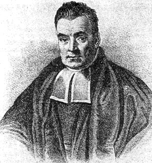
Thomas Bayes, in the portrait conventionally attached to his name. There is no verified likeness of Bayes; this image, from a 193690ya history of insurance, is of uncertain provenance and may not be him at all, which is a fittingly Bayesian situation to be in. (Public domain, via Wikimedia Commons.)
What Bayesian Inference Actually Is
Bayesian inference is the application of Bayes’ theorem to statistical problems. You start with a prior distribution encoding what you believe about some unknown parameters before seeing the data. You specify a likelihood function describing how the data would be generated given those parameters. Bayes’ theorem combines them into a posterior distribution, which is your updated belief after seeing the data.
\[P(\theta \mid D) = \frac{P(D \mid \theta) \, P(\theta)}{P(D)}\]
That is the whole thing. The posterior is proportional to the likelihood times the prior, and the denominator \(P(D)\), the marginal likelihood or “evidence,” is just the normalizing constant that makes it integrate to one. Everything else you have ever heard of in this field, Gibbs sampling, Hamiltonian Monte Carlo, variational inference, Stan, PyMC, is computational machinery for evaluating this formula when that denominator is an integral you cannot solve.
The philosophical appeal is that the posterior is your answer. You do not need to construct a confidence interval and then carefully avoid saying what everyone wants to say about it.3 A 95% credible interval actually means “there is a 95% probability the parameter lies in this interval,” given your model and prior. A 95% confidence interval does not mean that. It means that if you repeated the experiment infinitely many times, 95% of the intervals you constructed would contain the true parameter, which is a statement about the procedure, not about the particular interval in front of you. The Bayesian interpretation is the one humans actually want. The frequentist interpretation is the one the math supports. Most working scientists quietly use the first while officially reporting the second.
A Worked Example, Because the Abstraction Hides the Point
The formula is easy to state and easy to misunderstand, so here is the canonical example that makes it click. Imagine a medical test for a disease that 1 in 1,000 people have. The test is good: if you have the disease, it comes back positive 99% of the time, and if you do not, it comes back positive only 5% of the time. You take the test. It is positive. What is the probability you actually have the disease?
The intuitive answer most people give is somewhere around 95%, because the test is “95% accurate.” The correct answer is just under 2%. The reason is the base rate: the disease is so rare that the vast majority of positive results are false positives from the enormous healthy population. Out of 100,000 people, about 100 have the disease and test positive, while about 5,000 of the 99,900 healthy people also test positive. Your positive result is one of roughly 5,100, and only 100 of those are real. The prior, that ugly 1-in-1,000 starting point, dominates the answer even though the test is excellent.
This is the entire philosophy in one example. The likelihood (the test characteristics) is not enough. You have to combine it with the prior (how common the disease is) to get the thing you care about (the probability you are sick). Frequentist statistics is uncomfortable here because the “probability you have the disease” is not a long-run frequency; you either have it or you do not. Bayesian reasoning has no such discomfort. It treats your uncertainty as the object of study, which is what a patient sitting in the waiting room actually wants quantified.
This is also, not coincidentally, the structure of the raven paradox and most of the puzzles in philosophy of science about what counts as evidence. As one commenter put it in a Hacker News discussion of the paradox, “it makes a strong case for a system that integrates degree of confidence through and through, as opposed to merely assigning true and false.” That is the Bayesian pitch in a sentence. The world rarely hands you certainty, so build a framework that works in probabilities and updates as evidence arrives.
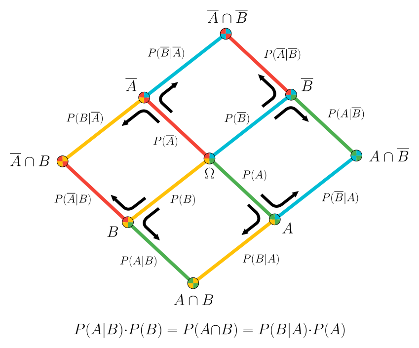
A 2D visualization of Bayes’ theorem: the posterior emerges from how the conditional regions overlap, not from the likelihood alone. (Qniemiec, CC BY-SA 3.0, via Wikimedia Commons.)
There is one subtlety worth flagging, because it bites people. Bayesian updating can produce certainty, by multiplying by zero. If your evidence has zero probability under a hypothesis, the posterior for that hypothesis is zero, permanently. This is why a recurring piece of folk wisdom among practitioners is to never assign a prior probability of exactly 0 or 1 to anything you might later want to reconsider. Assign zero and no amount of contrary evidence can ever move you. As one commenter on Hacker News noted, an infinitely confident prior “is impossible unless you have a screwy prior distribution.” Cromwell’s rule, named after Oliver Cromwell’s plea to “think it possible you may be mistaken,” is the formal version of this advice.
When Bayesian Methods Actually Help
I want to make the honest case here, which is narrower than the one you get from evangelists. There are situations where Bayesian inference is clearly the right tool, and there are situations where reaching for it is just signalling sophistication. Knowing the difference is most of the practical skill.
When you have genuine prior information. If you are estimating the effect of a new drug and you have results from twenty previous trials of similar drugs, incorporating that information through a prior is not just defensible, it is wasteful not to. Throwing away relevant evidence because your method has no slot for it is a strange thing to be proud of. et al 2004 lay out a careful framework for constructing priors from historical data in clinical trials, including the politically necessary trick of reporting results under a range of priors, from enthusiastic to skeptical, so reviewers can see how much the conclusion depends on prior belief.
When you need to quantify uncertainty in a way people can act on. Bayesian methods give you a full posterior distribution, not a point estimate and a p-value. You can answer questions like “what is the probability the effect is larger than the smallest clinically meaningful threshold?” directly, by integrating the posterior over that region. The frequentist framework cannot answer that question without contortions, because it does not assign probabilities to hypotheses at all.4
When the structure is hierarchical. Hierarchical models, where parameters at one level are themselves drawn from distributions whose parameters you also estimate, are natural in the Bayesian framework and genuinely hard to do well otherwise. Estimating individual school effects while accounting for district-level variation, modeling patient responses while borrowing strength across hospitals, combining heterogeneous studies in a meta-analysis: these are all hierarchical problems where partial pooling beats both complete pooling (ignore the groups) and no pooling (treat each group as an island). This connects directly to mixed-effects models, which are the frequentist cousin of the same idea. The classic teaching example, Efron and Morris’s analysis of 197056ya baseball batting averages, showed that shrinking individual estimates toward the group mean produced better predictions than each player’s own raw average. That result felt like a paradox in 197749ya. It is just partial pooling.
When your sample is small. With small samples, frequentist methods often produce absurd results: confidence intervals that include impossible values, maximum likelihood estimates pinned to the boundary of the parameter space, variance estimates of zero. Priors regularize the estimates, pulling them toward plausible values. This is mathematically the same operation as regularization in machine learning, and it helps for the same reason.5
When Bayesian Methods Don’t Help
The flip side deserves equal honesty, and you will not hear it often enough from people selling courses.
When you have a lot of data and vague priors. With large samples, the likelihood dominates the prior and Bayesian and frequentist answers converge. If you are analyzing 100,000 observations with a weakly informative prior, you will get essentially the maximum likelihood answer, just slower and with more ceremony. The Bernstein-von Mises theorem makes this precise: under regularity conditions the posterior concentrates around the MLE and becomes approximately normal as the sample grows. Using Bayesian machinery here because it is fashionable is a waste of compute and reviewer patience.6
When the prior is doing too much work. If your conclusions swing wildly with different reasonable priors, you do not have enough data to answer your question, and no amount of Bayesian machinery will rescue you. The fix is to run a sensitivity analysis across a range of priors and report it. If the result is not robust, say so plainly. The failure mode to avoid is choosing the prior after seeing the data to get the answer you wanted, which is “prior hacking,” the Bayesian cousin of p-hacking and just as corrosive.7
When the computation does not converge and you cannot tell. This is the objection I find most persuasive, and it is the one practitioners actually run into. On a thread about Statistical Rethinking, a commenter going by civilized put it bluntly: “The biggest problem with Bayesian statistics in practice is the frequent reliance on relatively slow, unreliable methods such as MCMC. The Bayesian methodology community loves to advocate for packages like Stan, claiming that they make Bayesian stats easy. This is true, relative to Bayesian stats without Stan. But these packages are often much, much harder to get useful results from than the methods of classical statistics. You have to worry about all sorts of technical issues specific to these methodologies, because these issues don’t have general technical solutions.” That is not a strawman from a frequentist partisan. It is a fair description of what it feels like to debug a model that will not mix.
The Computational Reality
The dirty secret of applied Bayesian statistics is that most of the difficulty is not philosophical, it is numerical. You wrote down a beautiful model. Now you have to actually compute the posterior, and the posterior is a high-dimensional probability distribution you can evaluate only up to a constant. There is no closed form. So you sample.
Markov chain Monte Carlo is the family of algorithms that does this. The idea, going back to the Metropolis algorithm from the 195373ya Los Alamos work on the hydrogen bomb, is to build a random walk through parameter space that visits each region in proportion to its posterior probability.8 Run it long enough and the samples it produces are draws from the posterior, which you can then summarize however you like. Gibbs sampling is a special case that updates one parameter at a time and was the workhorse of the 1990s through tools like BUGS. Modern tools mostly use Hamiltonian Monte Carlo, which borrows ideas from physics to take large, informed steps through the space instead of the small random shuffles of older methods, and which is dramatically more efficient on the correlated, awkwardly-shaped posteriors that real models produce.
The catch is that none of this is push-button. MCMC can fail to converge, and worse, it can fail to converge while looking like it converged. The chain can get stuck in one region, or two chains can settle into different answers, or the sampler can quietly fail to explore the tails where the action is. This is why diagnostics are not optional. You check R-hat, which compares variance within and between chains and should sit below about 1.01; you check the effective sample size, which tells you how many genuinely independent draws you have after accounting for autocorrelation; and you stare at trace plots looking for chains that have not mixed. In HMC specifically, “divergent transitions” are a loud warning that the sampler is choking on the posterior’s geometry, usually in hierarchical models with tight funnels, and the standard fix is reparameterization rather than just running longer.
There is a real cost here that the textbooks undersell. A logistic regression that a frequentist fits in milliseconds might take a Bayesian model minutes to sample, and a complex hierarchical model can run for hours and still hand you divergences you have to diagnose by hand. One commenter captured the tradeoff cleanly: when you have few parameters, gradient descent is “smoking fast,” but once you want full uncertainty quantification rather than a point estimate, you are paying for Monte Carlo, and that bill grows with the model. Whether the uncertainty is worth the wait is a judgment call you have to make every time.
The 2026 Toolkit, and How to Choose
The practical Bayesian stack has consolidated. If you are starting today, you do not need to survey the whole zoo; you need to pick one of these four and learn it well.
Stan is the reference implementation for general-purpose Bayesian inference. It uses the No-U-Turn Sampler, an adaptive form of HMC, and it is the most battle-tested sampler in the field. You write models in Stan’s own language and call them from R, Python, or Julia. One quirk worth knowing, raised by a Stan developer on Hacker News: Stan is fp64 (double precision) throughout, which makes it less suited to the low-precision GPU hardware that deep learning is built around. It is a CPU-first tool, and proudly so.
PyMC is Python-native and feels more natural if you live in the NumPy ecosystem. You build models with ordinary Python context managers, and it does both MCMC and variational inference. As one commenter argued, PyMC is “more powerful and concise than training a model in Stan” for many workflows, though Stan’s sampler still has an edge in robustness on hard posteriors.
brms is an R package that compiles Stan code from lme4-style formula syntax. If you can write
y ~ x + (1 | group), you can fit a Bayesian hierarchical model in one line. This is the fastest path from curiosity to a fitted model, and it is where I usually tell people to start.NumPyro is built on JAX and is fast, especially with GPU acceleration. It is increasingly the choice when Bayesian inference meets large-scale machine learning, where you want autodiff and hardware acceleration in the same framework.
These are all probabilistic programming languages: you describe the generative model and the system figures out the inference. That separation, model here, inference there, is the real engineering achievement of the last twenty years, and it is what turned Bayesian statistics from a craft into something closer to a tool.
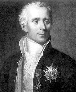
Pierre-Simon Laplace, who did most of the actual work of turning Bayes’s drawer-essay into a working theory of inference, and who arguably deserves the name. Portrait after Sophie Feytaud. (Public domain, via Wikimedia Commons.)
The Prior Problem, Which Is Smaller Than It Looks
The standard objection to Bayesian inference, the one you will hear within thirty seconds of mentioning it to a frequentist, is the prior. “Your results depend on subjective assumptions.” This is true. It is also less damning than it sounds, and the reason is worth dwelling on.
Frequentist methods embed assumptions too. The choice of sampling model, which covariates to include, what functional form to assume, whether to log-transform, where to set the significance threshold: these are all consequential choices, and they receive far less scrutiny precisely because nobody labels them “subjective.” 2017 argue that the objective/subjective dichotomy is a red herring. All statistical inference involves choices. The honest question is not whether your analysis is free of assumptions, because none are, but whether the assumptions are stated openly and defended. Bayesian methods at least force the prior into the open. Frequentist methods bury equivalent commitments inside model specification, where they are harder to audit.
The Hacker News discussions on this are, for once, genuinely illuminating, because the same fight has been had a thousand times by people who do this for a living. One camp insists Bayesian methods are “just as subjective,” since two analysts with different priors fed the same evidence reach different conclusions. The sharper response, from a commenter named btilly, reframes it: “Bayesian statistics are not subjective at all. Instead they objectively describe the correlation between prior belief and conclusion. People may draw different conclusions for subjective reasons, but that subjectivity is in the people, not the statistics.” The update rule is mechanical and shared. What you bring to it is yours. That is not a bug, it is an accurate description of how evidence works, and another commenter, yummyfajitas, drew out the practical implication: a lab reporting a diagnostic result should arguably hand you an update rule, “whatever your prior estimate is, multiply it like so,” rather than a single posterior probability that silently bakes in the lab’s own prior.
In practice, the way working statisticians have defused this whole argument is the weakly informative prior. Instead of either an “uninformative” prior (which is harder to specify coherently than it sounds, and often is not actually uninformative) or a strongly opinionated one, you use a prior that rules out the absurd while staying agnostic about the plausible. A prior of Normal(0, 10) on a standardized regression coefficient says, in effect, “effects this large are physically impossible, but within the realm of the possible I am not going to lean.” et al 2008 and the Stan prior choice recommendations are the practical references here, and they have done more to make Bayesian analysis routine than any philosophical argument ever did.
Where Bayes Actually Shows Up
It is easy to talk about this abstractly, so here is where the machinery earns its keep in the world, often without anyone calling it Bayesian.
Clinical trials. This is where the prior argument stops being academic. Regulators including the FDA now accept Bayesian designs, especially adaptive trials that update their allocation as data arrive and platform trials testing many treatments at once. The appeal is concrete: you can borrow strength from earlier phases, stop early when the posterior is decisive, and report “the probability this drug beats placebo by a clinically meaningful margin” instead of a p-value nobody interprets correctly. Rare-disease trials, where you will never have a large sample no matter how long you wait, are close to the ideal case. The cost, as always, is that the prior is now load-bearing and has to be pre-specified and defended.
Machine learning, quietly everywhere. The connection runs deep. Gaussian processes are Bayesian by construction. Bayesian optimization is the standard method for tuning expensive hyperparameters, because it reasons about uncertainty to decide where to evaluate next. Variational autoencoders are built on variational inference. Even mainstream deep learning keeps bumping into Bayesian ideas: dropout has a Bayesian interpretation, weight decay is a Gaussian prior, and Bayesian neural networks remain an active research line precisely because everyone wants calibrated uncertainty out of models that are currently overconfident. The link to overfitting and regularization is not an analogy, it is the same math wearing different clothes.
A/B testing and the web. A surprising amount of Bayesian inference happens inside product analytics. Bayesian A/B testing lets you ask “what is the probability variant B beats variant A?” directly, and crucially lets you peek at results as they come in without the multiple-comparisons penalties that make frequentist sequential testing painful. One HN commenter described working out “the exact probability that B is better than A” by integrating the posterior directly, no normal approximation required, which is exactly the kind of small-sample situation where the Bayesian answer is cleaner. Multi-armed bandit algorithms, which power recommendation and ad systems, are often Thompson sampling under the hood, which is Bayes all the way down.
Spam filters and the original killer app. Before any of this was fashionable, the naive Bayes classifier was quietly filtering your email. Paul 2002 essay “A Plan for Spam” popularized Bayesian spam filtering, and for years it was most people’s only contact with the method. It is “naive” because it pretends features are independent, which they are not, and it works anyway, which is a useful lesson about when modeling assumptions can be wrong in theory and fine in practice.9
A Workflow, Not a Ritual
If there is one thing I want you to take from this, it is that running MCMC and reporting a posterior is the middle of the job, not the whole of it. et al 2020 describe a full Bayesian workflow, and the steps that bracket the actual fitting are the ones that separate trustworthy analysis from elaborate self-deception.
Prior predictive checks. Before touching the data, simulate datasets from your prior alone. If your prior happily generates negative human heights or treatment effects of fifty standard deviations, it is too vague, and you have learned that before it could mislead you.
Fit and check diagnostics. R-hat, effective sample size, divergent transitions. If the sampler did not converge, nothing downstream means anything, so this is a gate, not a formality.
Posterior predictive checks. Simulate data from the fitted posterior and compare it to the real data. If your model cannot reproduce the obvious features of the data you already have, it is misspecified, and you should fix the model rather than admire its credible intervals.
Sensitivity analysis. Refit under a few defensible alternative priors. Report how much the conclusion moves. If it moves a lot, the data are not speaking loudly enough and you should say so.
Model comparison done right. Use leave-one-out cross-validation or WAIC, not Bayes factors, which are notoriously sensitive to prior specification in exactly the regions where it is hard to think clearly.
This is more work than a t-test, and it should be. The extra effort buys better-calibrated uncertainty and conclusions you can actually defend, but only if you do all of it. Doing step two and skipping the rest gives you the false confidence of sophistication without the substance, which is arguably worse than an honest t-test.
So Should You Be a Bayesian?
The framing of the question is the mistake. After spending real time with both toolkits, I have come to think the Bayesian-versus-frequentist culture war is mostly a relic, kept alive by textbooks and Twitter rather than by anyone doing serious applied work. The professionals I find most credible are fluent in both and choose by problem. Lots of data and a question about long-run error rates? Frequentist tools are fast and well-understood. Small samples, real prior information, hierarchical structure, or a decision that needs an honest probability attached? Reach for Bayes.
What I will defend without hedging is the epistemology. Bayesian reasoning is the correct account of how beliefs should change in response to evidence, and that is true whether or not you ever fit a model in Stan. The base-rate example is not a statistical curiosity, it is a thinking tool that prevents a specific, common, expensive error. Internalizing “update from a prior, in proportion to the evidence, and never let your confidence hit exactly zero or one” makes you better at reasoning about medical tests, forecasts, and your own pet theories, regardless of which software you open on Monday.
The honest summary is the boring one. Bayesian inference is a powerful, sometimes essential, often overkill set of tools, attached to a genuinely excellent way of thinking about uncertainty. It is not a revolution and it is not a religion. It is plumbing, with unusually good philosophy bolted on. Learn when the plumbing is worth installing, keep the philosophy with you always, and ignore anyone trying to sell you the whole thing as a worldview.
This essay draws on community discussions from Hacker News threads on Bayesian statistics, Stan, and probabilistic programming, with technical claims verified against primary sources. For the deeper texts, McElreath’s Statistical Rethinking is the best practitioner’s introduction, Gelman et al’s Bayesian Data Analysis is the comprehensive reference, and the Bayesian Workflow paper is the methodological backbone of the workflow section. Related pieces on this site: Bayesian vs. Frequentist, Effect Sizes vs. P-Values, Mixed-Effects Models, Meta-Analysis Methods, and Overfitting and Regularization.