Diffusion Models
From thermodynamics to text-to-image: how diffusion models work, why they displaced GANs, and the messy path from DDPM to Stable Diffusion. The forward process destroys; the reverse process creates.
- Diffusion Models
- The Forward Process: Structured Destruction
- The Reverse Process: Learning to Create
- Score Matching: the Other Perspective
- From DDPM to the Real World
- The Text-To-Image Explosion
- Why Diffusion Won, and What People Thought about It
- Beyond Images
- The Parts That Are Still Broken
- Where This Leaves Us
- Further Reading
Diffusion Models
The idea is almost perverse in its simplicity. Take a clean image, destroy it by adding noise step by step until nothing is left but static, then train a neural network to reverse the destruction. Generation is just running the reverse process starting from pure noise. That is the whole trick behind diffusion models, the class of generative models that between 2020 and 2024 went from an academic curiosity to the dominant approach in image generation, and increasingly in video, audio, and 3D too. Along the way they displaced GANs, VAEs, and basically everything else that came before.
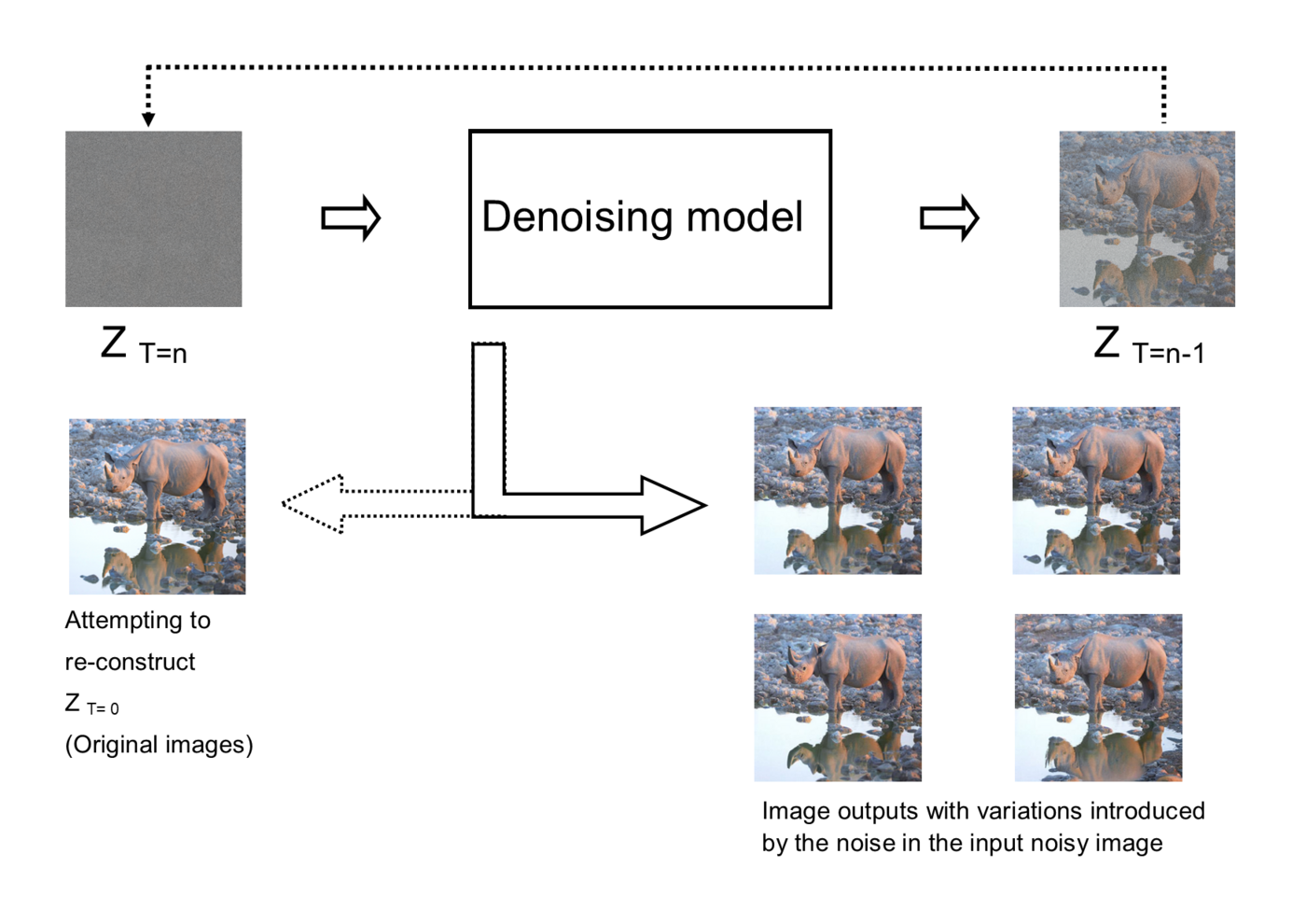
A diffusion model denoising a sample step by step: pure Gaussian noise on the left, gradually resolving into a coherent image on the right. The reverse process is just this, run a thousand times. (Image: Wikimedia Commons, CC BY-SA 4.0)
What makes diffusion models remarkable is not just that they produce better images, though they do. It is that they get there through a training procedure that is almost embarrassingly dumb. No adversarial training, no mode collapse, no delicate equilibrium between a generator and a discriminator that you have to babysit for a week. You just predict the noise. The theoretical machinery underneath that simplicity runs deep, though: non-equilibrium thermodynamics, score matching, stochastic differential equations, and variational inference all converge on the same framework from different directions. Understanding diffusion models means understanding why those perspectives are the same thing, and why that sameness turns out to be useful rather than just elegant.
I find this one of the more satisfying corners of modern machine learning, precisely because the gap between the practice and the theory is so wide. A graduate student can implement a working diffusion model in an afternoon. Explaining why it works can fill a semester. Most of the time in deep learning the theory lags far behind what works; here the theory is rich and the practice is trivial, and somehow they meet in the middle.
The Forward Process: Structured Destruction
The forward process, also called the diffusion process or the noising process, is not learned. It is defined analytically, by hand, with no parameters to fit. Given a data sample \(\mathbf{x}_0\) drawn from the data distribution \(q(\mathbf{x}_0)\), we define a sequence of increasingly noisy versions \(\mathbf{x}_1, \mathbf{x}_2, \ldots, \mathbf{x}_T\) by adding Gaussian noise at each step:
\[q(\mathbf{x}_t | \mathbf{x}_{t-1}) = \mathcal{N}(\mathbf{x}_t; \sqrt{1 - \beta_t}\,\mathbf{x}_{t-1}, \beta_t \mathbf{I})\]
Here \(\beta_t \in (0, 1)\) is a noise schedule that controls how much noise gets added at step \(t\). Typically \(\beta_t\) grows from something small (around \(10^{-4}\)) to something larger (around \(0.02\)) over \(T\) steps, with \(T\) on the order of 1000. By step \(T\) the signal has been almost entirely obliterated, and \(\mathbf{x}_T\) is approximately an isotropic Gaussian with no memory of the original \(\mathbf{x}_0\).1
A crucial property makes all of this tractable. You can sample \(\mathbf{x}_t\) directly from \(\mathbf{x}_0\) without grinding through every intermediate step. Defining \(\alpha_t = 1 - \beta_t\) and \(\bar{\alpha}_t = \prod_{s=1}^{t} \alpha_s\):
\[q(\mathbf{x}_t | \mathbf{x}_0) = \mathcal{N}(\mathbf{x}_t; \sqrt{\bar{\alpha}_t}\,\mathbf{x}_0, (1 - \bar{\alpha}_t)\mathbf{I})\]
That closed form is what makes training efficient. You do not simulate the forward process one step at a time. You jump straight to any noise level \(t\) and compute the corrupted image in one shot. This is the computational shortcut that makes training on millions of images feasible instead of absurd. Without it, every training step would require a thousand sequential noise additions, and the whole enterprise would be a non-starter.
The forward process is, mathematically, a discrete approximation to an Ornstein-Uhlenbeck process, a well-studied stochastic process that gradually forgets its initial condition and settles into a Gaussian stationary distribution. Sohl-Dickstein et al. (201511ya) first proposed using this thermodynamic framing for generative modeling, drawing explicitly on the physics of diffusion. The connection to non-equilibrium statistical mechanics is not just a metaphor someone reached for in the introduction. The math is literally the same.2 That 201511ya paper sat mostly ignored for five years, which is its own small lesson about how research timing works. The idea was right. The execution and the compute were not there yet.
The Reverse Process: Learning to Create
The generative model is the reverse of the forward process. Starting from noise \(\mathbf{x}_T \sim \mathcal{N}(0, \mathbf{I})\), we iteratively denoise our way back to a clean sample \(\mathbf{x}_0\). The reverse process is parameterized as:
\[p_\theta(\mathbf{x}_{t-1} | \mathbf{x}_t) = \mathcal{N}(\mathbf{x}_{t-1}; \boldsymbol{\mu}_\theta(\mathbf{x}_t, t), \sigma_t^2 \mathbf{I})\]
The neural network \(\boldsymbol{\mu}_\theta\) predicts the mean of the denoised distribution at each step. The variance \(\sigma_t^2\) can be fixed or learned. In practice, fixing it to \(\beta_t\) or to \(\tilde{\beta}_t = \frac{1 - \bar{\alpha}_{t-1}}{1 - \bar{\alpha}_t}\beta_t\) works well enough that nobody loses sleep over it.3
The critical insight from Ho et al. (2020), the DDPM paper, was a reparameterization. Instead of predicting the mean \(\boldsymbol{\mu}_\theta\) directly, the network predicts the noise \(\boldsymbol{\epsilon}_\theta(\mathbf{x}_t, t)\) that was added to turn \(\mathbf{x}_0\) into \(\mathbf{x}_t\). The training objective collapses to something almost insultingly clean:
\[\mathcal{L}_{\text{simple}} = \mathbb{E}_{t, \mathbf{x}_0, \boldsymbol{\epsilon}}\left[\|\boldsymbol{\epsilon} - \boldsymbol{\epsilon}_\theta(\mathbf{x}_t, t)\|^2\right]\]
That is the whole loss. Sample a training image \(\mathbf{x}_0\), sample a random timestep \(t\), sample random noise \(\boldsymbol{\epsilon}\), compute the noisy image \(\mathbf{x}_t\), predict the noise with the network, minimize the squared error. It is a regression problem, conceptually no harder than denoising a photo, which is one of the oldest problems in computer vision. The genuinely surprising part is that doing this across all noise levels at once trains a full generative model. You set out to build a denoiser and you accidentally build something that can dream.
Score Matching: the Other Perspective
There is a second, arguably deeper, way to understand diffusion models, through the lens of score matching. The score of a distribution \(p(\mathbf{x})\) is the gradient of its log-density, \(\nabla_{\mathbf{x}} \log p(\mathbf{x})\). A score-based model learns to estimate this gradient field and then uses it to generate samples via Langevin dynamics, iteratively walking uphill along the score with a bit of added noise at each step.
Song & Ermon (2019) showed you could train score-based models using denoising score matching: estimate the score of the noised distribution at various noise levels. Song et al. (2021) then unified the score-based and diffusion perspectives by showing they are both special cases of stochastic differential equations. The forward process is an SDE that diffuses data into noise. The reverse process is another SDE that runs backward in time, and its drift term involves precisely the score \(\nabla_{\mathbf{x}_t} \log q(\mathbf{x}_t)\).
This unification matters because it reveals that predicting the noise \(\boldsymbol{\epsilon}\), as DDPM does, is equivalent to estimating the score. Concretely, \(\nabla_{\mathbf{x}_t} \log q(\mathbf{x}_t | \mathbf{x}_0) = -\frac{\boldsymbol{\epsilon}}{\sqrt{1 - \bar{\alpha}_t}}\). The noise-prediction network and the score network are the same object up to a scaling factor. That is why the literature uses the two terms almost interchangeably. They are literally the same function, viewed through two different theoretical windows.4 I remember finding this genuinely disorienting the first time it clicked, the way you feel when two friends from completely different parts of your life turn out to already know each other.
The SDE Framework in Detail
Song et al. (2021) formalized diffusion models as continuous-time stochastic processes. The forward process is described by an SDE:
\[d\mathbf{x} = \mathbf{f}(\mathbf{x}, t)\,dt + g(t)\,d\mathbf{w}\]
where \(\mathbf{f}\) is a drift coefficient, \(g\) is a diffusion coefficient, and \(\mathbf{w}\) is a Wiener process. For the variance-preserving formulation used in DDPM, \(\mathbf{f}(\mathbf{x}, t) = -\frac{1}{2}\beta(t)\mathbf{x}\) and \(g(t) = \sqrt{\beta(t)}\).
The reverse-time SDE, established by Anderson (198244ya), is:
\[d\mathbf{x} = \left[\mathbf{f}(\mathbf{x}, t) - g(t)^2 \nabla_{\mathbf{x}} \log q_t(\mathbf{x})\right]dt + g(t)\,d\bar{\mathbf{w}}\]
where \(\bar{\mathbf{w}}\) is a reverse-time Wiener process. The only unknown is the score \(\nabla_{\mathbf{x}} \log q_t(\mathbf{x})\), which is exactly what the neural network learns to approximate.
This continuous formulation buys you several things. First, you can derive the probability flow ODE, a deterministic version of the reverse SDE that traces the same marginal distributions without any stochastic noise. This ODE enables exact likelihood computation via the instantaneous change-of-variables formula, making diffusion models proper density estimators, which is something GANs never were. Second, the continuous view lets you use adaptive ODE solvers for generation, choosing the number of steps dynamically based on how much quality you want. DDIM (Song et al., 2020) was an early version of this idea, a deterministic sampler that could produce decent images in 50 steps instead of 1000.
The probability flow ODE also connects diffusion models to normalizing flows, via continuous normalizing flows, and to optimal transport theory. Those connections got exploited by flow matching (Lipman et al., 2022), which sidesteps the SDE framework entirely and directly learns a vector field that transports noise to data along straighter paths. Flow matching has become increasingly popular through 2025 and 2026, partly because it tends to enable faster generation with fewer steps. The newest open-weight image models lean on it heavily.
From DDPM to the Real World
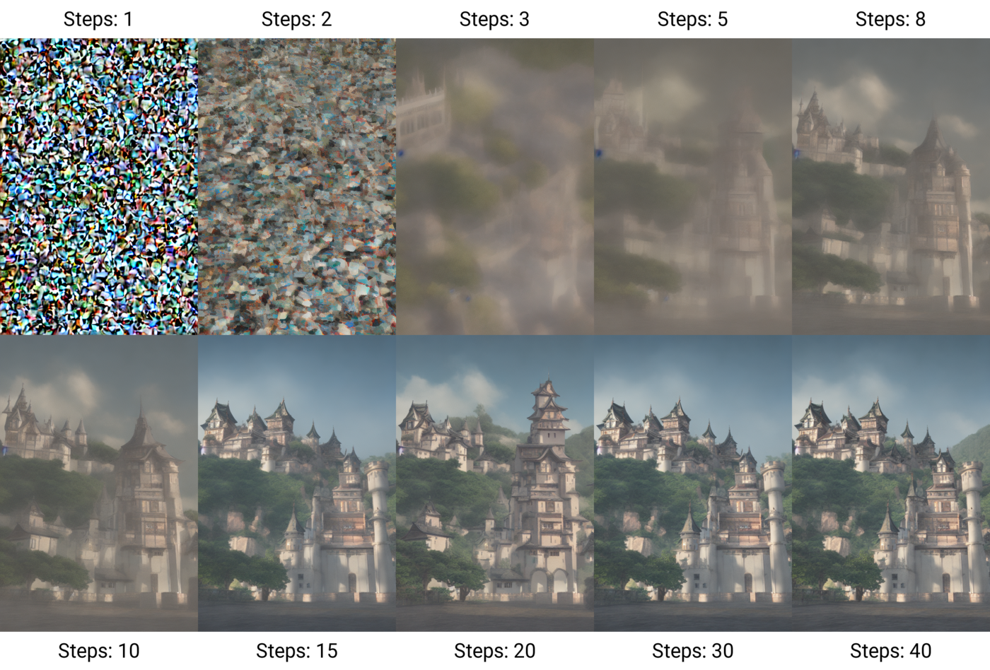
Samples generated with DDIM at different step counts. More steps generally means higher fidelity, but the returns flatten fast, which is why 20 to 50 step samplers became standard. (Image: Wikimedia Commons, CC BY-SA 4.0)
Ho et al. (2020), DDPM, showed that diffusion models could generate high-quality 256x256 images competitive with GANs. But the road from “competitive research result” to “anyone can generate photorealistic images from text on a laptop” needed several more breakthroughs, none of which were obvious at the time.
Improved architectures. Dhariwal & Nichol (2021) showed that diffusion models could actually beat GANs on FID and other image-quality metrics, using a better U-Net with attention layers, adaptive group normalization, and classifier guidance, a technique that trades diversity for quality by nudging sampling with a classifier’s gradients.5 The title of that paper, “Diffusion Models Beat GANs on Image Synthesis,” reads now like a small declaration of war, and it turned out to be accurate.
Classifier-free guidance. Ho & Salimans (2022) killed the need for a separate classifier by training the diffusion model both conditionally and unconditionally, then extrapolating between the two at inference time. This became the standard conditioning mechanism. Nearly every text-to-image model uses classifier-free guidance with a guidance scale \(w\) that sets the tradeoff between fidelity to the prompt and sample diversity. Crank it up and you get images that hew tightly to your words but start to look oversaturated and samey. Dial it down and you get variety at the cost of “did it even read my prompt.”6
Latent diffusion. The single most important engineering insight came from Rombach et al. (2022): do not run diffusion in pixel space. Compress images into a lower-dimensional latent space with a pretrained autoencoder, run diffusion there, then decode back to pixels. This cut computational cost by roughly an order of magnitude. The resulting latent diffusion model architecture became Stable Diffusion, which, trained on LAION-5B and released with open weights, democratized image generation in a way no previous model had. The weights fit on a consumer GPU. That single fact changed the entire trajectory of the field.7
Faster sampling. Thousand-step generation is unusable in practice. A long line of work, including DDIM, DPM-Solver, and consistency models (Song et al., 2023), pushed the required steps from 1000 down to 50, then 20, then in the limit a single step. Consistency models pull this off by directly learning a map from any point on the diffusion trajectory back to its origin, trading a little quality for the ability to generate in one forward pass.
The Text-To-Image Explosion
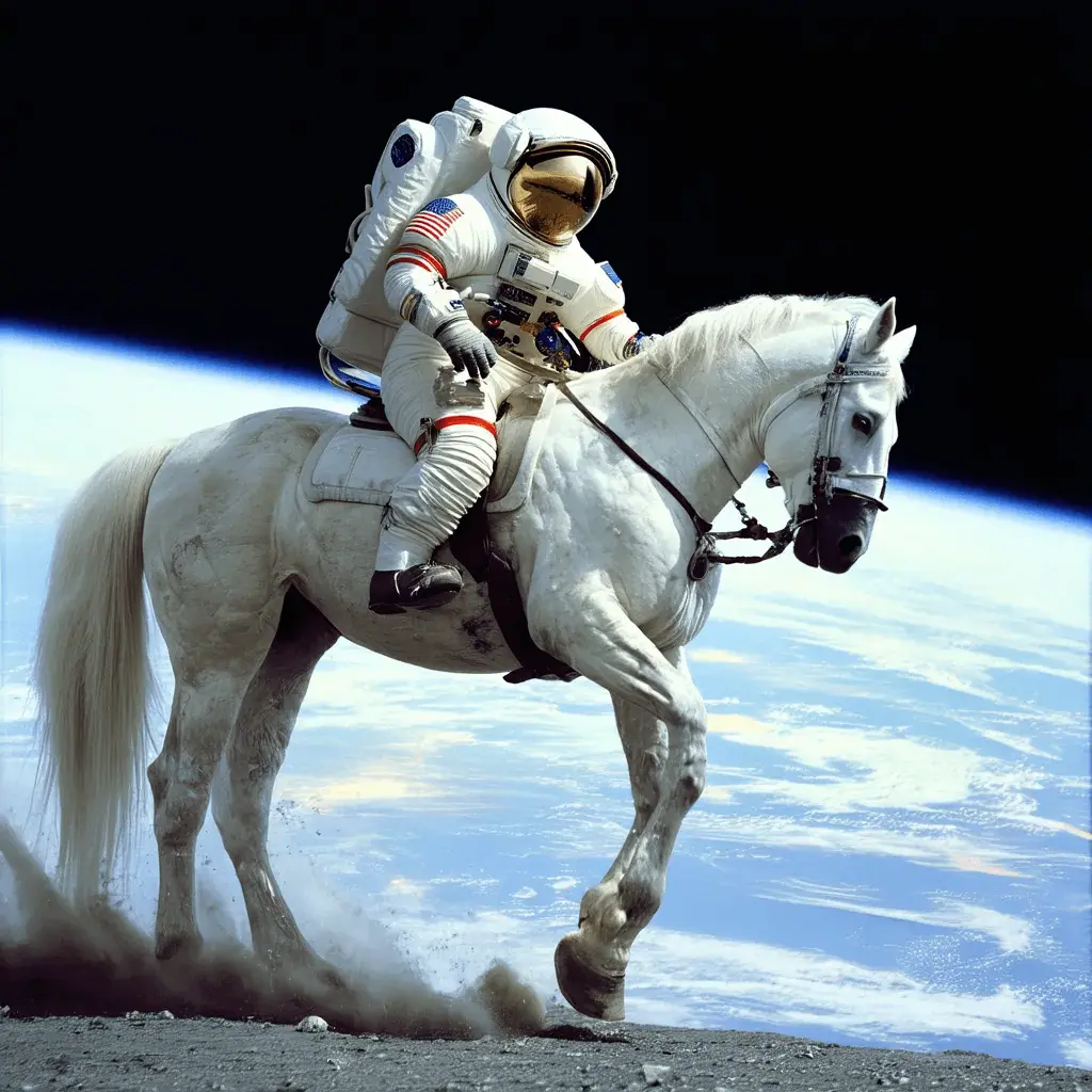
A 1024x1024 sample in the style that became instantly recognizable in 2022: a photorealistic subject rendered from a short text prompt. The aesthetic of these models is now so familiar it is almost invisible. (Image: Wikimedia Commons, CC BY-SA 4.0)
For most people the word “diffusion” means none of the math above. It means typing a sentence and getting a picture. That capability arrived in a roughly twelve-month window in 2022 that, looking back, was one of the strangest years in the history of machine learning. DALL-E 2 from OpenAI landed in April, Imagen from Google in May, Midjourney opened its beta in July, and Stable Diffusion shipped open weights in August. By the autumn, generating images that would have looked like science fiction eighteen months earlier was something a teenager could do for free on a Discord server.
What made these models work was not diffusion alone. It was diffusion plus a way to steer it with language. DALL-E 2 used a CLIP text encoder to turn a prompt into an embedding, then a diffusion “prior” and “decoder” to turn that embedding into an image. Imagen made a finding that surprised a lot of people: a giant frozen language model, a T5 text encoder trained only on text, produced better image-text alignment than a model trained jointly on image-caption pairs. The text understanding mattered more than anyone expected. Google’s own paper reported that scaling the text encoder improved sample fidelity more than scaling the image diffusion model itself, which is a genuinely odd result if you think the hard part is the pixels.8
Then there is the part of the story that the research papers leave out. Stable Diffusion’s open release did something the closed models structurally could not. Within weeks there was a sprawling ecosystem: web UIs, fine-tuning scripts, a flood of community checkpoints, and an economy of shared model weights traded on sites like Civitai. As one Hacker News commenter, nylonstrung, described that world: “Everything is using Stable Diffusion as underlying model, then most of the usage is merged of checkpoints.” Another, satvikpendem, noted that “regular people too are using them to make posters and invitation cards.” The base model was a starting point, not a product. People bent it toward whatever they wanted, and the speed at which they did it caught even the researchers off guard.
Why Diffusion Won, and What People Thought about It
It is worth being precise about what diffusion models beat, because “they make prettier pictures” undersells it. Before 2020 the state of the art in image generation was GANs, and GANs had a reputation among the people who actually trained them. They were fast at inference, which mattered, but training them was a known misery. Mode collapse, where the generator quietly decides to produce only a handful of outputs that reliably fool the discriminator, was a constant threat. Getting a GAN to converge on a new dataset could take a researcher weeks of babysitting learning rates and praying. Diffusion models swapped all of that for a stable regression loss that essentially always trains. You give up inference speed and you get back your sanity. For a field where a single training run can cost real money, that trade was worth making.9
The reaction outside research circles was more complicated, and more interesting. The democratization argument cut both ways. satvikpendem, watching the later anxiety about AI coding tools, drew the parallel sharply: “exact same argument that occurred when Stable Diffusion released, but engineers on HN didn’t really care as long as it made pretty pictures. But now that AI comes for my industry? Oh the outrage! In reality it’s just hypocrisy all around.” That stuck with me, because it is partly true and partly unfair, and the part that is true is uncomfortable. A lot of the people who cheered when image generation undercut illustrators went quiet about the principle when their own livelihoods came into view.
There was also a strain of pure technical wonder that I think gets lost in the culture-war framing. The Animats comment captures it: faced with a grand claim about the mystery of human insight, he wrote, “Go watch Stable Diffusion iteratively transform noise into originality.” Whatever you think about the economics, there is something legitimately uncanny about watching static resolve into a coherent scene, step by step, because a network learned the gradient of a probability density. The first time you run the reverse process and watch an image assemble itself out of nothing, it does not feel like statistics. It feels like a magic trick whose method you happen to know.
Beyond Images
If diffusion models only made pictures, they would still be a big deal. But the framework turned out to be almost embarrassingly general. The recipe, destroy structured data with noise, learn to reverse it, is indifferent to what the data actually is, and over the past few years it has colonized one domain after another.
Video. Text-to-video is the obvious next frontier, and it is much harder, because you have to keep an image coherent not just in space but across time. OpenAI’s Sora, Google’s Veo, and a wave of open models treat video as a diffusion problem over space-time latents. Temporal consistency is the recurring failure mode. Objects flicker, hands do impossible things, a coffee cup teleports across a table between frames. The trajectory is the same one image models walked from 2020 to 2023, just a couple of years behind and with a much larger compute bill.
Audio. Diffusion handles waveforms and spectrograms well. Models in this space generate speech, music, and sound effects, and the same denoising machinery applies whether the data is pixels or amplitudes over time.
Molecules and proteins. This is the application that I find most quietly important. Diffusion models that operate on 3D atomic coordinates have become a serious tool in structural biology and drug discovery. RFdiffusion designs novel proteins by denoising backbone structures, and AlphaFold3 (2024) replaced the architecture of its predecessor with a diffusion-based module for predicting molecular structure. When a generative technique developed to make anime avatars ends up designing candidate enzymes, you are watching a genuinely general idea propagate through science. The same gradient-of-log-density trick works on a probability distribution over folded proteins.10
Other modalities. People have applied diffusion to 3D shapes, point clouds, tabular data, robot trajectories, and even, in a loop back to the field’s center of gravity, to text. Diffusion language models try to generate text by denoising rather than the left-to-right autoregression that Transformers use. Whether they will ever beat autoregressive models at language is an open and contested question. The Hacker News commenter Bolwin was blunt about the practical catch with parallel-decoding approaches: “Parallel decoding may be great if you have a nice parallel gpu or npu but is dog slow for cpus.” The general lesson of the last few years is that you should not bet against diffusion in a new domain too confidently, but language is the one place where the incumbent is very, very strong.
The Parts That Are Still Broken
I want to resist the tidy narrative where diffusion models solved generation and everyone lived happily. They did not, and the unsolved problems are revealing.
The first is speed, which is the original sin of the whole approach. Autoregressive samplers and GANs generate in one or a few passes. A naive diffusion model needs hundreds. Every advance from DDIM through DPM-Solver to consistency models has been, at bottom, a fight against the iterative nature of the reverse process. The progress is real, single-step and few-step generation now exist, but it usually comes with a quality tax, and the fact that so much of the field’s effort goes into not running the algorithm as designed should tell you the design has a fundamental tension in it.
The second is that these models do not understand the things they draw. They are extraordinary at texture and lighting and composition, and they are famously bad at anything requiring a world model: counting objects, getting the number of fingers right, rendering legible text in an image, respecting that a prompt asked for a red cube on top of a blue sphere rather than the reverse. Compositional reasoning, binding the right attribute to the right object, remains shaky even in the best 2026 models, because the model is matching the statistics of its training data rather than reasoning about a scene. It is a very sophisticated stylist with no idea what it is depicting.
The third set of problems is not technical at all, and it is the one that will outlast the others. Stable Diffusion and its peers were trained on LAION-5B, a dataset of billions of image-text pairs scraped from the open web, with no consent from and no payment to the artists whose work was in it. The lawsuits followed quickly. Getty Images sued Stability AI; a group of artists filed a class action; the legal questions about whether training on copyrighted images is fair use are, as of 2026, still genuinely unsettled and working their way through courts on two continents. There are also the darker externalities: the same tools generate non-consensual imagery and floods of synthetic media, and the LAION dataset itself was found to contain illegal material and had to be pulled and cleaned. None of this is a footnote to the technology. The training-data question is the technology, because a generative model is in a real sense a lossy compression of its training set, and you cannot cleanly separate “the math is elegant” from “the math was fit to a corpus of other people’s work.”
I find I hold two thoughts at once here, and I have stopped trying to collapse them. The technical achievement is real and beautiful. The way it was built and deployed ran roughshod over a lot of people who had no say in it. Both things are true, and the second does not become false because the first is impressive.
Where This Leaves Us
Diffusion models are, to me, the cleanest recent example of how progress in machine learning actually happens, which is almost never the way the textbook tells it afterward. The core idea sat in a 2015 paper that almost nobody read. It needed a reframing (noise prediction), an engineering trick (latent space), a conditioning method (classifier-free guidance), and an open release before it became the thing that ate image generation. Each of those was a separate insight by separate people, years apart, and none of them was obvious in advance. The thermodynamics was right in 201511ya. The world just was not ready to use it.
What stays with me is the strange double nature of the thing. Underneath, it is some of the most elegant mathematics in modern ML, with score matching, stochastic differential equations, and variational inference all turning out to be three views of the same object. On top, it is a regression loss so simple you could explain it to a first-year student in five minutes. And the output is a machine that turns sentences into pictures, noise into faces, randomness into something that, against all reason, looks like meaning. I have been doing this long enough to be hard to impress. This still does.
Further Reading
Generative Adversarial Networks, the approach diffusion models displaced, and why training them was such a pain
Transformer Architecture, the backbone of the text encoders that made text-to-image work
Foundation Models, the broader shift that diffusion image models are part of
The Scaling Hypothesis, on why scaling the text encoder mattered more than the image model
Lilian Weng’s “What are Diffusion Models?”, the single most-recommended technical explainer, repeatedly cited in community threads
“Understanding Diffusion Models: A Unified Perspective” (Luo, 2022), a careful walk through the variational and score-based derivations
This piece draws on Sohl-Dickstein et al. (201511ya) on the original thermodynamic framing; Ho et al. (2020), the DDPM paper; Song et al. (2021) on the SDE unification; Rombach et al. (2022) on latent diffusion; the Wikipedia entry on diffusion models; and practitioner discussion on Hacker News. Images are from Wikimedia Commons under the licenses noted in each caption.