Neural Scaling Laws
Power laws govern everything in deep learning: loss falls as a power of compute, data, and parameters. From Kaplan’s original observations through Chinchilla’s correction to the evidence that scaling bends, breaks, and occasionally lies.
There is an empirical regularity in neural network training that, once you see it, you cannot unsee. Plot the loss against compute, data, or parameters on a log-log scale and you get a straight line. Not approximately straight. Not sort-of-straight-if-you-squint. Straight, over many orders of magnitude. That straight line is a power law, and it is the closest thing deep learning has to a law of nature.
\[L(X) = \alpha X^{-\beta} + L_\infty\]
Here \(X\) is the resource you are spending (compute \(C\), data \(D\), or parameters \(N\)), \(\alpha\) and \(\beta\) are fitted constants, and \(L_\infty\) is the irreducible loss: the entropy of the data itself, the floor below which no model can go regardless of scale.1 This functional form turns up in language modeling, image classification, machine translation, speech recognition, protein folding, and even game-playing agents. It is unreasonably universal, and nobody fully understands why.
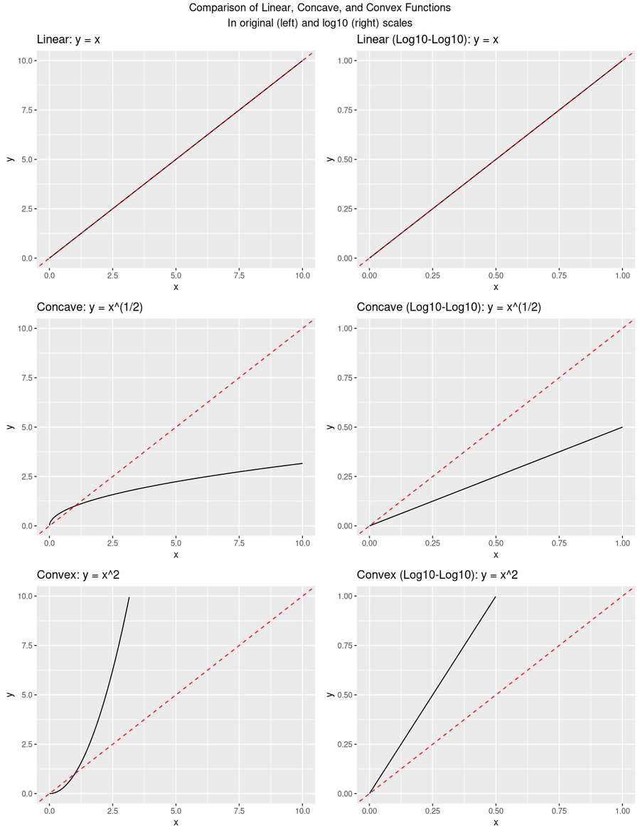
Power-law curves in linear scale (top) and on a log-log scale (bottom), where they become straight lines. This is the visual signature of every neural scaling result. Image by Wikimedia Commons user Talgalili, CC BY-SA 4.0.
I want to be honest about my relationship with this topic up front, because it colors everything that follows. I find scaling laws both the most exciting and the most deflating result in modern machine learning. Exciting because they make a famously unpredictable field predictable: you can fit a curve on small models and forecast what a model 100 times larger will do, often to within a few percent. Deflating because the lesson they teach is that a great deal of progress came not from cleverness but from spending. The curve does not care how elegant your idea is. It cares how many FLOPs you fed it.
That tension is the whole story. Scaling laws are why labs will spend fifty million dollars on a single training run without flinching, because they are not hoping it works, they are predicting it will. And they are why a lot of thoughtful people now wonder whether the field has been mistaking a budget line for a research program.
Kaplan Et Al.: the Discovery
The modern story starts with Kaplan et al. (2020), a paper from OpenAI that systematically measured how language model loss depends on model size, dataset size, and compute budget. They trained a large family of Transformer language models, from tiny ones up to over a billion parameters, and measured cross-entropy loss. Across all three axes, the relationship was a clean power law.
The headline findings were these. Loss falls as a power of parameter count, roughly \(L(N) \propto N^{-0.076}\) for models trained to convergence. It falls as a power of data, roughly \(L(D) \propto D^{-0.095}\), for models large enough not to be capacity-bottlenecked. And it falls as a power of compute, roughly \(L(C) \propto C^{-0.050}\), which is the most useful of the three because compute is what you actually budget for. They also found that within the Transformer family, total parameter count dominated the specific tradeoff between width and depth.2
The most consequential claim was about how to spend a fixed compute budget. Kaplan et al. argued you should pour most of it into making the model bigger rather than training it on more data. They recommended scaling parameters faster than tokens, roughly \(N \propto C^{0.73}\) and \(D \propto C^{0.27}\). The implication: optimal models should be enormous and trained on comparatively little data for comparatively few steps. That conclusion shaped GPT-3 and, through it, the strategy of the entire field.3
There was something intoxicating about this. It suggested that capability, or at least the next-token-prediction proxy we use for it, has a simple and predictable relationship with resources. No phase transitions, no mysterious walls, just the steady grind of exponential investment buying polynomial improvement. On Hacker News, the venture investor gdiamos put it well when comparing the scaling bet to a doomed-but-instructive chip startup: “Sometimes the only way to get to the bottom of a complex system is to build it. The same could be said of scaling laws and LLMs. It was theory before Dario, Ilya, OpenAI, et al trained it.” That is the part people forget. Before 2020 the idea that bigger was reliably better was a hunch. Kaplan turned the hunch into a measured curve, and a measured curve is something you can raise money against.
Chinchilla: the Correction
Then Hoffmann et al. (2022), the “Chinchilla” paper from DeepMind, showed that Kaplan had the allocation badly wrong.
The Chinchilla team trained more than 400 models from 70M to 16B parameters, varying model size and data size together rather than holding one fixed. They found the compute-optimal split was far more balanced than Kaplan claimed. Parameters and data should scale at roughly the same rate with compute. Double your budget, and you should spend about half of it on more parameters and about half on more tokens.4
The punchline landed hard: most large language models in existence were significantly undertrained. GPT-3, at 175B parameters trained on 300B tokens, should have seen something closer to 3.7 trillion tokens to be compute-optimal. Gopher, at 280B parameters on 300B tokens, was worse. The Chinchilla model itself, a mere 70B parameters trained on 1.4T tokens, beat the 280B Gopher despite being a quarter of the size, simply because it was fed almost five times as much data.
The practical fallout was immediate and large. A compute-optimal 70B model is cheaper to serve than a compute-equivalent 280B model, because inference cost tracks parameter count, not training compute. The whole industry had been building models that were needlessly expensive to run. LLaMA was designed explicitly around Chinchilla-style scaling and showed that smaller, better-trained models could match much larger ones. The gwern.net proprietor gwern, commenting on HN, captured how total the shift was: PaLM-1 “is hobbled by the fact that it was probably the largest (because the last) LLM to be trained with the Kaplan scaling laws rather than the Chinchilla. As soon as Chinchilla came out, no one would train like PaLM-1 again, because it was giving up so much performance.” When a result retroactively makes the largest model anyone built look like a mistake, you know it mattered.
Why did Kaplan get it wrong? The reason is subtle and worth sitting with, because it is a cautionary tale about experimental design. Kaplan et al. used a fixed learning rate schedule across model sizes. That meant their smaller models were never fully trained: when training stopped, their learning rate was still too high, so they looked worse than they should have. The bias made larger models appear disproportionately good, which pushed the recommendation toward “go bigger.” Hoffmann et al. used three independent estimation methods and got consistent answers from all three. The correction was not a matter of taste. It was a fixed bug in how the first experiment was run.
That fact alone should make anyone humble about the next scaling law that gets declared. The field’s most influential allocation rule was off by a wide margin for two years, propagated into billions of dollars of training runs, and the error came down to a learning-rate schedule. I think about that whenever someone quotes scaling exponents to three decimal places as if they were physical constants. They are fitted parameters from a particular experimental setup, and setups have bugs.
The Anatomy of a Scaling Law
It is worth pausing on what these power laws are actually saying, because the math constrains the interpretation more than people assume.
A power law \(L \propto N^{-\beta}\) means each multiplicative increase in \(N\) buys a constant multiplicative decrease in the excess loss \(L - L_\infty\). Going from \(10^9\) to \(10^{10}\) parameters cuts excess loss by the same factor as going from \(10^{10}\) to \(10^{11}\). The absolute gain shrinks at every step while the cost grows linearly or worse. This is the iron law of scaling. You are on a treadmill that gets more expensive with every stride.5
The exponents are everything. Kaplan’s \(\beta \approx 0.076\) for parameter scaling means you need on the order of \(10^{13}\) times more parameters to halve the excess loss. That is an absurd number. The compute exponent near 0.050 is worse still. These tiny exponents explain both why scaling works, because it is smooth and predictable, and why it is unsatisfying, because the returns are polynomial while the bills are exponential. When aspenmartin argued on HN that you cannot have a coherent conversation about LLM progress without knowing “what chinchilla scaling laws are,” the snark was a little much, but the underlying point holds: the shape of the curve sets the terms of every debate about whether we are near a wall.
There is a deeper question lurking here. Why power laws at all? Several theoretical frameworks have been proposed, and I find all of them partially convincing and none of them sufficient.
One family of explanations comes from statistical mechanics. Sharma and Kaplan (2022) connect the scaling exponent to the intrinsic dimension of the data manifold: if the data lives on a manifold of dimension \(d\), the loss should fall like \(N^{-\alpha/d}\), with \(\alpha\) depending on how smooth the target function is. A second comes from compression. Hutter (2021) derives power-law scaling from first principles by treating a network as a lossy compressor of the data distribution, which ties the whole thing to rate-distortion theory. A third comes from feature learning dynamics, where Bordelon et al. (2024) model the curve as a spectral decomposition: features are learned roughly in order of decreasing variance, and each new feature contributes a little less than the last.6
The honest summary is that we observe power laws, we can fit them, we can predict with them, and we lack a first-principles theory convincing enough to tell us when they will break. That gap is not academic. The entire question of how much further scaling can take us hinges on a phenomenon we can measure but cannot derive.
When Scaling Breaks
And break it does, or at least bend. The clean power-law story has been complicated by a series of observations that make the picture richer, and in some ways less optimistic, than the smooth curves suggest.
Start with emergent abilities. Wei et al. (2022) documented capabilities that appear abruptly at certain model scales rather than improving gradually: multi-step arithmetic, chain-of-thought reasoning, some kinds of code generation. Tasks that sat at chance for small models jumped to high accuracy inside a narrow scaling window. If real, this is bad news for extrapolation, because you cannot forecast a discontinuity from a smooth fit. I cover this in more depth in the piece on emergent abilities, but the short version is that the story got more interesting in 2023.
Schaeffer et al. (2023) argued, convincingly to my eye, that a lot of emergence is a measurement artifact. Use a harsh, discontinuous metric like exact-match accuracy and a gradual improvement in the underlying probability distribution can look like a sudden leap. Switch to a continuous metric like log-probability of the correct answer and the jump mostly smooths out. The capability was improving steadily the whole time; the metric manufactured the cliff. This won a NeurIPS best-paper award, and it deserved to, but I would not treat it as the final word.7
Next, not everything scales at the same rate. Caballero et al. (2023) showed that individual benchmarks can have wildly different exponents, and some tasks barely improve with scale at all because they are bottlenecked by something other than raw capability. Precise factual recall, certain flavors of mathematical reasoning, and formal verification tend to plateau far earlier than next-token loss would lead you to expect. The aggregate curve is smooth; the per-task curves underneath it are a mess.
Then there is the gap between pretraining loss and what you actually care about. The relationship between low loss and good downstream behavior is looser than the literature sometimes implies. Reinforcement learning from human feedback, instruction tuning, and chain-of-thought prompting can all shift the effective curve, sometimes a lot. A smaller model with good post-training can beat a larger one with worse post-training even though the larger model has lower pretraining loss. This is part of why the Chinchilla-optimal recipe has itself been superseded in practice: labs now routinely over-train well past the compute-optimal point, because the inference savings from a smaller model dominate the extra training cost, and post-training can paper over the slightly higher loss.8
Finally, and most importantly for where the field is heading, you can trade inference-time compute for capability, and that trade has different scaling properties than pretraining. Snell et al. (2024) and the broader test-time-compute movement showed that best-of-N sampling, search, and extended chains of thought can buy performance that complements pretraining scale. For reasoning-heavy tasks the inference-time exponents look better than the pretraining ones, meaning you sometimes get more out of letting a model think longer than out of training a bigger one.9 This is the insight behind reasoning models, and it reopened the scaling frontier just as people were starting to worry it was closing.
The Data Wall
Here is the problem that keeps the people running these labs up at night. The Chinchilla recipe says you should feed a model roughly 20 tokens for every parameter. Push that recipe to the model sizes people now want to train and you run out of text. Villalobos et al. (2024) estimated that frontier models will exhaust the entire stock of publicly available, reasonable-quality human-generated text somewhere between 2026 and 2032, with a central estimate around 2028. The internet is large but it is finite, and the fraction of it worth training on is smaller than the raw byte count suggests.
This is the data wall, and it changes the character of the whole enterprise. For most of the 2010s the binding constraint was compute. You always had more data than you could afford to train on, so the game was buying GPUs. Chinchilla quietly flipped that. Once you are supposed to scale data and parameters in lockstep, and once the highest-quality data is the part you run out of first, data becomes the thing you cannot just buy. You can always rent more accelerators. You cannot rent another internet.
The reaction on Hacker News has the resigned quality of people watching a known deadline approach. Discussing a paper on self-adapting models, khalic summarized the standard framing: “Villalobos et al. project that frontier LLMs will be trained on all publicly available human-generated text by 2028. We argue that this impending ‘data wall’ will necessitate the adoption of synthetic data augmentation. Once web-scale corpora is exhausted, progress will hinge on a model’s capacity to generate its own high-utility training signal.” That is the optimistic read: when you run out of human text, you make a model write more.
I am skeptical of the synthetic-data escape hatch, and so are a lot of practitioners. Training a model on its own output risks model collapse, where errors compound across generations and the distribution narrows until the model forgets the tails it was supposed to learn. There are ways around this, mostly involving keeping a strong anchor of real data and using synthetic data to augment rather than replace, but nobody has shown that you can scale purely synthetic generation the way you scaled web scraping. The honest position is that the data wall is real, the workarounds are partial, and the smooth extrapolations everyone draws past 2028 are doing a lot of quiet assuming.
There is a subtler version of the worry too. Even if you do not literally run out of text, the marginal token gets worse. The first trillion tokens you scrape are Wikipedia, books, and well-edited prose. The tenth trillion is forum spam, machine-translated junk, and increasingly the output of earlier language models. Data quality is itself a scaling axis, and it is one where the curve probably bends down as you go, in exactly the regime where Chinchilla says you need more.
Is It Actually a Law?
I want to push on the word “law,” because it does a lot of rhetorical work and I think it is partly a sleight of hand. A law in physics is a statement that holds because of something deeper: conservation of energy, the structure of spacetime, the statistics of large ensembles. A neural scaling law is a curve fit. It describes a regularity we have observed over a finite range of scales, in a particular architecture, on a particular kind of data. Calling it a law borrows the authority of physics for what is, so far, a stable-looking empirical trend.
The HN commentariat is sharper on this than the press releases. janalsncm put the objection bluntly, warning against “LLM maximalist ideas that suggest infinite ‘scaling laws’ for LLMs (they are not laws), leading to ridiculous conclusions like building a $1 trillion cluster is the fastest way to AGI.” The parenthetical is the whole argument. A power law fit over six orders of magnitude tells you nothing guaranteed about the seventh. Every extrapolation past the measured range is a bet that no new bottleneck appears, and the history of the field is mostly a history of new bottlenecks appearing.
There is also a slippery thing about how the laws get used. The functional form is robust, but the constants are not portable. The same aspenmartin who insisted you need to know the math also posted the actual fitted form from Chinchilla, \(L(N,D) \approx 1.69 + 406.4/N^{0.34} + 410.7/D^{0.28}\), with the caveat that the constants “change and are domain and model specific.” That caveat matters more than the equation. The exponents people quote come from one data distribution and one architecture family. Change the tokenizer, change the data mix, change the architecture, and you refit everything. The shape survives; the numbers do not. So “the scaling law predicts X” usually means “a curve we fit on our data, assuming our setup generalizes, predicts X,” which is a much weaker claim than the phrasing implies.
None of this means scaling laws are useless. They have made genuinely correct predictions about large training runs, which is more than most of machine learning theory can say. But there is a difference between “this is a reliable engineering tool within the regime where we have data” and “this is a law of nature that licenses trillion-dollar extrapolations.” The first is true. The second is marketing. I think a lot of the discourse, and a meaningful fraction of the capital, has been operating on the second when only the first is earned. The deeper case for why bigger keeps working at all, independent of the specific curves, is what I take up in the scaling hypothesis; here I only want to flag that the curve and the hypothesis are different claims and deserve different levels of confidence.
What Scaling Bought, and What It Didn’t
It would be churlish not to admit how much scaling delivered. The jump from GPT-2 to GPT-3 to GPT-4 was mostly scale, and it took language models from amusing autocomplete to tools that millions of people use for real work. In-context learning, the ability to pick up a task from a few examples in the prompt without any weight updates, was not designed in. It fell out of making the model bigger. Whatever you think about the limits, the empirical fact is that a remarkable amount of capability came from turning one knob.
But scaling has been notably bad at certain things, and the pattern of failures is informative. Reliable arithmetic on large numbers does not come from scale; it comes from tools or from teaching the model to use a scratchpad. Faithful factual recall does not scale the way fluency does, which is why even enormous models still hallucinate confidently. Out-of-distribution generalization, the thing we actually mean when we say “reasoning,” improves with scale but slowly and unevenly, and a lot of apparent reasoning turns out to be sophisticated pattern matching that breaks when you change surface details that should not matter.
This is the part I find genuinely hard to think about. The scaling curve is smooth, so it is tempting to read it as a smooth approach to general intelligence. But the curve is measuring loss, and loss is dominated by the easy, frequent cases. A model can drive its average loss down impressively while the hard, rare cases that we care most about barely move. The aggregate metric improves; the specific failures persist. That gap between what the curve measures and what we want is, I think, the central unresolved tension in the whole scaling story, and no amount of additional compute obviously closes it.
The 2024-2025 pivot to inference-time compute is partly an admission of this. When DeepSeek’s results suggested you could get strong reasoning out of pure reinforcement learning and more thinking time rather than a bigger base model, the framing among optimists was telling. As kiratp put it, it “means we now have a clear path to just keep throwing more compute at the problem,” only now the compute goes into the model’s reasoning at inference time rather than into its parameter count at training time. The treadmill did not stop. It just moved.
The Math, for the Curious
If you want the actual machinery, the cleanest statement is the joint Chinchilla form. Loss is modeled as a sum of three terms: an irreducible floor, a parameter term, and a data term.
\[L(N, D) = E + \frac{A}{N^\alpha} + \frac{B}{D^\beta}\]
Here \(E\) is the entropy of natural text, the loss you would get from a perfect model. The \(A/N^\alpha\) term is the cost of having finite capacity; it vanishes as the model grows. The \(B/D^\beta\) term is the cost of having finite data; it vanishes as you train on more tokens. Hoffmann et al. fit \(E \approx 1.69\), \(\alpha \approx 0.34\), \(\beta \approx 0.28\), with the constants \(A\) and \(B\) in the low hundreds.
To find the compute-optimal allocation, you fix the compute budget. For a Transformer, training compute is approximately \(C \approx 6ND\), where the factor of 6 counts the floating-point operations per token for a forward and backward pass.10 Then you minimize \(L(N, D)\) subject to \(6ND = C\) using a Lagrange multiplier. Because \(\alpha\) and \(\beta\) are close to equal, the optimum puts roughly equal effort into \(N\) and \(D\): both scale as approximately \(C^{0.5}\). That is the entire content of “scale parameters and data together.” It is one constrained optimization on a three-term curve.
Kaplan’s analysis used a different parameterization and, crucially, did not fully decouple the learning-rate schedule from model size, which is how the two papers reached different exponents from overlapping data. The lesson worth carrying away is that the headline recommendation of a scaling paper is downstream of a dozen fitting choices, and reasonable-looking choices produced a two-year, industry-wide error.
Where This Leaves Me
I have come to think of scaling laws as the most important boring discovery in modern AI. Boring because the underlying message is “spend more and you get a bit more, predictably.” Important because that predictability is what turned a research curiosity into an industry, and because the exact shape of the curve, the tiny exponents, the irreducible floor, the data wall, sets hard limits on how far the spending can go.
What I keep returning to is the duality. The optimist reads the straight line on the log-log plot and sees a ramp to general intelligence, smooth and reliable, just keep climbing. The pessimist reads the same line and sees diminishing returns made mathematically explicit, a polynomial payoff against an exponential bill, with a data wall at the end of the runway. Both are looking at the same curve. The curve does not adjudicate between them, because it only describes the regime we have measured, and the disagreement is entirely about the regime we have not.
My own position, for whatever it is worth, is that scaling is real, it is slowing in the ways the math predicts it should, and the recent excitement about inference-time compute is a genuine new axis rather than a continuation of the old one. We learned to predict loss. We did not learn to predict capability, and the gap between those two is where all the interesting arguments still live. The curve is a tool, a good one, and like every good tool it is most dangerous when people mistake it for a prophecy.
Primary sources: Kaplan et al., “Scaling Laws for Neural Language Models” (2020); Hoffmann et al., “Training Compute-Optimal Large Language Models” (Chinchilla, 2022); Villalobos et al., “Will we run out of data?” (2024); Wei et al., “Emergent Abilities of Large Language Models” (2022); Schaeffer et al., “Are Emergent Abilities a Mirage?” (2023); Snell et al., “Scaling LLM Test-Time Compute” (2024). Community discussion from Hacker News, quoted with attribution and linked inline. Related essays on this site: the scaling hypothesis, the Transformer architecture, emergent abilities, in-context learning, and foundation models.