Backpropagation: The Chain Rule That Ate Machine Learning
A first-person account of backpropagation: its prehistory, the priority dispute, what the 1986 paper did and did not invent, the math, and the alternatives people keep proposing.
- Backpropagation: The Chain Rule That Ate Machine Learning
- The Chain Rule Is Older Than Your Grandfather’s Neural Network
- Linnainmaa and the Reverse Mode Nobody Talked About
- Werbos, 197452ya And 1982
- 1986: The Paper Everyone Remembers
- LeCun and the Zip Codes
- The Winter, the Revival, and the Controversy
- The Math, Without Hand-Waving
- Why It Still Matters
- The Beyond-Backprop Literature
- What I Think
- Conclusion
- Further Reading
- Citation
Backpropagation: The Chain Rule That Ate Machine Learning
Every time I start a training run, I trigger an algorithm whose core idea fits on a napkin, and which I cannot fully explain without a whiteboard. I call loss.backward() and a few hundred milliseconds later every weight in a model with billions of parameters has a gradient. I rarely think about what happened. That is probably the correct amount of thought for a working engineer, and it is also a kind of hazard. The algorithm underneath, backpropagation, is the thing that made deep learning practical, and most people who use it could not tell you who invented it, when, or what the original authors actually claimed.1
This essay is my attempt to answer those questions honestly, and to say what I think about them. The short version: backpropagation is not really “the chain rule applied to neural networks,” although that is how it is usually introduced, and it is not the invention of any single person in 198640ya, although that is how it is usually remembered. It is a particular efficient way of computing gradients in a computational graph, discovered at least once in a different context, rediscovered several times, and then finally noticed by the right community at the right moment with the right hardware. The history is messier and more interesting than the textbook version, and the priority fights are real, though I think they are less important than they look.
I will go through the prehistory, the 197056ya reverse-mode paper that everyone in the automatic differentiation community already knows about, the 197452ya and 198244ya work of Paul Werbos, the 198640ya paper by Rumelhart, Hinton and Williams that broke the field open, and the 198937ya LeCun work that showed the method could read zip codes. Then I will spend some time on the math, because I think the math is where most of the understanding lives, and finally I will look at the “beyond backprop” literature that has grown up over the last few years, since it is the best evidence that people are still unhappy with the algorithm. I should flag at the outset that I have not been able to read the 198640ya Nature paper’s text or the 198937ya LeCun PDF in full; where I describe their content I am relying on bibliographic checks and on secondary accounts, and I say so.2
The Chain Rule Is Older Than Your Grandfather’s Neural Network
The starting point is the chain rule of calculus, which says that the derivative of a composition of functions is the product of the derivatives of its parts. Written out for a nested function, \(\frac{d}{dx} f(g(x)) = f'(g(x)) \, g'(x)\). Leibniz is credited with a version of this notation in 1676350ya, and Schmidhuber’s account, which I will return to repeatedly, traces a chain-rule-based approach to the sensitivity of a composed system back to that period and to L’Hôpital’s textbook in 1696330ya.3 I have not checked these primary sources myself, so I treat them as part of the secondary history rather than as settled fact. The idea that a derivative of a composition can be assembled from local derivatives is about as old as calculus itself, and there is nothing controversial about that.
The step from “the chain rule exists” to “we can train machines by propagating errors backward” took much longer, and it went through control theory rather than through neural networks. In the late 1950s and early 1960s, engineers working on optimal control of rockets, aircraft and other dynamical systems needed to compute how a performance index changed when they perturbed a trajectory. The method of steepest descent applied to such trajectories is the conceptual ancestor of what we now do with weights. Henry 1960 paper on the gradient theory of optimal flight paths, Arthur 1961 work, Stuart 1962 simplified derivation via the chain rule, and the 196957ya textbook of Bryson and Ho all sit in this lineage.4 The thing to notice is that these people were not doing machine learning. They were doing optimal control, where the “network” is a discretized trajectory and the “parameters” are the controls at each time step. The backward sweep that computed the gradient was a practical necessity for guiding a physical vehicle, not a metaphor for learning.
Meanwhile, two other threads were developing in parallel. The first is stochastic approximation, which goes back to the Robbins and Monro paper of 195175ya and gives us the theoretical footing for updating parameters from noisy gradient estimates. Almost every training run today is a descendant of the stochastic gradient descent idea that comes from this work, and the fact that we are still using it, with only small modifications, is a striking piece of evidence that the basic idea was right. The second thread is the perceptron. Frank Rosenblatt’s perceptron in the late 1950s had a learning rule that adjusted weights according to errors, but it was a single layer with a hard threshold, and it could not represent functions like XOR. The famous criticism in Minsky and Papert’s 196957ya book Perceptrons was devastating for single-layer networks, and it was also, in a way, a warning: the obvious fix was to add layers, but nobody had a good way to train the hidden layers, because the error signal was not directly available there.
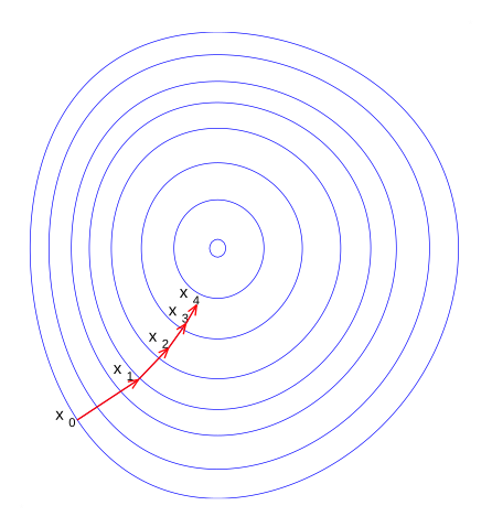
An illustration of the gradient descent method: each step moves downhill, against the gradient, toward a minimum of the loss. Illustration by Zerodamage, public domain, via Wikimedia Commons.
The key observation for the rest of the story is this. To train a multilayer network with a gradient method, you need the derivative of the loss with respect to every weight, including weights deep in the network whose outputs never reach the loss directly. That is precisely the credit assignment problem in its most mechanical form. You can compute these derivatives by brute force, perturbing each weight and re-running the network, which costs one forward pass per parameter. Or you can notice that the chain rule lets you reuse intermediate results, and organize the computation so that a single backward sweep gives you all the gradients at once. The second approach is what people now mean by backpropagation, and its history is largely the history of who noticed it, and in what form.
Amari’s 196759ya work is worth a mention here, because it is often cited as one of the first examples of training a multilayer perceptron end to end by stochastic gradient descent, with the hidden representation being learned rather than fixed.5 The details of that work are not something I can check in this essay, and I would not want to lean on any particular claim about its exact algorithm. What I think is safe to say is that, by the late 1960s, the pieces existed in various places: gradient-based optimization, the chain rule, layered networks, and a growing sense that hidden layers were the crux of the matter. What did not yet exist was the efficient reverse-mode computation, applied to a neural network, that put them together.
Linnainmaa and the Reverse Mode Nobody Talked About
The work that is most often cited as the first general formulation of what we now call backpropagation is Seppo Linnainmaa’s 197056ya master’s thesis at the University of Helsinki. The thesis is hard to access directly for most readers, and the case for its importance rests mostly on the account Schmidhuber gives in his history pages and surveys, which cites the FORTRAN code and the relevant pages of the thesis.6 The journal version that I can verify with more confidence is 1976 paper in BIT Numerical Mathematics, volume 16, pages 146 to 160, with the DOI 10.1007/BF01931367. Its title is, to put it mildly, not what a machine learning researcher would expect: “The representation of the cumulative rounding error of an algorithm as a Taylor expansion of the local rounding errors.” The paper is about numerical analysis, specifically how rounding errors accumulate in a computation. The reverse-mode idea appears there as a method for computing those error terms efficiently, by sweeping backward through the computation.
This is the key technical point, and it is the reason I think the reverse mode deserves more credit in the story than it usually gets. Consider a function \(f: \mathbb{R}^n \to \mathbb{R}\), which is the typical case for a loss function with many parameters. Forward-mode differentiation computes one directional derivative per pass, so getting the full gradient costs \(n\) passes. Reverse-mode differentiation computes the full gradient in a single backward pass, at a cost comparable to a constant multiple of evaluating the function itself. For a neural network with millions of weights and a scalar loss, the difference is the difference between an algorithm that is useless and one that is practical. Linnainmaa’s contribution, as I understand it, was to write down this reverse accumulation in general form and to show that it gives derivatives of an arbitrary differentiable program, rather than only of specific formulas.
The modern name for this technique is reverse-mode automatic differentiation, and the person who has done the most to make the history of that name clear is Andreas Griewank. In a 201214ya article in Documenta Mathematica, titled, appropriately enough, “Who invented the reverse mode of differentiation?”, Griewank traces the idea through the numerical analysis and computational science literature.7 His paper is more careful than most priority essays I have read, and it makes the important point that “inventing” the reverse mode and “applying it to neural networks” are very different achievements. The first is a numerical method. The second is a decision about what to do with the method.
Schmidhuber argues that Linnainmaa’s work should be credited as the origin of backpropagation, and he has a point. The 197056ya thesis and the 197650ya paper do contain the essential computational structure. I am skeptical, though, of the implied claim that Linnainmaa was doing what we would call training a neural network. He was doing numerical analysis of rounding error, and the mapping to gradient-based learning of weights is something a reader has to supply. This is a common pattern in the history of ideas, and it is worth being explicit about. An algorithm can exist, be correctly described, and be published, long before anyone sees its application. The question “who invented backprop?” is therefore partly a question about which application you consider definitive. If you define backpropagation as the reverse-mode gradient computation, Linnainmaa is the clear answer. If you define it as the use of that computation to train multilayer networks, the answer moves forward in time.
I also want to flag that Schmidhuber’s own account includes a 197155ya journal publication by Ostrovskii and coauthors as one of the early appearances of related ideas.8 I have not verified that claim independently, and I would treat it the way I treat most priority claims in this area: as a lead to check, not as a finding.
Werbos, 197452ya And 1982
The next major figure is Paul Werbos. 1974 PhD thesis at Harvard, which Schmidhuber discusses in some detail, is often cited as the first explicit proposal to use the backward propagation of derivatives to train what he called a neural network model.9 The thesis, as I understand the accounts that cite it, applies the reverse computation to a model of learning with a sensitivity analysis, and Werbos explicitly discusses the idea of applying it to multilayer structures. Whether the 197452ya thesis is “backpropagation for neural networks” in the sense that matters is a question on which the secondary literature disagrees, and I think the fair summary is that Werbos’s thesis is a clear step in that direction, though not yet the application that became standard.
The clearer milestone is 1982 paper, “Applications of advances in nonlinear sensitivity analysis,” which appeared in a volume of the IFIP conference proceedings published by Springer.10 This is the paper that Schmidhuber and others point to as the first application of the reverse computation specifically to neural networks in a form that a modern reader would recognize. I should stress that I have not read the paper, and my description of its content is a summary of how it is cited, not my own reading.
What I find most interesting about the Werbos story is not the priority question but the reception. Werbos’s ideas were available, cited, and published in the early 1980s, and they did not catch on in the way the 198640ya paper did. There are several plausible explanations. The computing power was not there to make the experiments compelling. The problems people were trying to solve, mostly small pattern recognition tasks, did not obviously need hidden layers. And the broader field was still in a state where the perceptron critique loomed large. Ideas do not spread because they are correct. They spread because a particular group of people, in a particular venue, with a particular set of demonstrations, makes them seem like the next obvious step. That is what happened in 198640ya.
1986: The Paper Everyone Remembers
The paper that most people mean when they say “backpropagation was invented in 1986” is Rumelhart, Hinton and Williams’s “Learning representations by back-propagating errors,” published in Nature in volume 323, pages 533 to 536, in October of that year, with DOI 10.1038/323533a0.11 I was able to verify the bibliographic metadata through Crossref. What I was not able to do is read the text, because the paper is paywalled and the PDF that I could fetch has no extractable text layer. So I will describe what I think the paper did, with the caveat that my description is based on how it is cited and on the general history, not on a line-by-line reading. I will not quote it.
As I understand it, the paper’s contribution was not the invention of the reverse computation. It was a clean, short statement of the method for training multilayer networks with differentiable units, together with a set of demonstrations showing that the hidden units learn internal representations that capture meaningful structure in the data. The title itself is telling. The phrase “learning representations” points at the thing that made the paper matter: the claim that a network trained this way does not merely fit a function, it learns features. That is the idea that connects backpropagation to everything that came after, from speech recognition to the embeddings in large language models.
Schmidhuber’s framing, which I take seriously but do not fully accept, is that the 198640ya paper was a popularization of ideas that had already been published, and that its authors did not cite the earlier work carefully enough.12 There is some evidence for the second part. Discussions of the paper’s citations, including the way Werbos’s work is handled, have been contentious for decades. But I think the first part is misleading. Popularization is not a minor achievement. A paper that makes an idea legible to a large community, with clear notation, a convincing set of experiments, and the right venue, does something that an obscure thesis does not. If the test of priority were only who first wrote the equations, we would have to credit a long list of people, and most of them would have no idea what the field would become.
My own view is that the 198640ya paper deserves the reputation it has, but for reasons that are more specific than “inventing backprop.” It reframed the question from “can we train multilayer networks?” to “what do hidden units learn?” It gave the community a vocabulary, and it gave the emerging connectionist movement a demonstration that could be reproduced by others. Those are real contributions, and they are the kind of contributions that determine how a field develops. Credit for the algorithm belongs to a longer chain of people. Credit for making it the default way of thinking about learning belongs in large part to these three authors.
LeCun and the Zip Codes
1986 was the moment the idea became legible, 198937ya was the moment it became useful in a way that people outside the academic neural network community could see. Yann LeCun and his coauthors published “Backpropagation Applied to Handwritten Zip Code Recognition” in Neural Computation, volume 1, issue 4, pages 541 to 551, in 1989, with DOI 10.1162/neco.198937ya.1.4.541.13 I verified the bibliographic metadata. The PDF that I could download is a scanned document with no extractable text, so again I cannot quote it, and my description is based on the paper’s standard citation and on the well-known history of convolutional networks.
The significance of this paper, as I understand it, lies in its combination of architecture and training. The network is a convolutional design, with local receptive fields and shared weights, and it is trained end to end with backpropagation on a real-world task: recognizing handwritten digits from postal codes. The architecture encodes a prior about images, namely that local patterns matter and that the same feature detector is useful at every location. The training algorithm finds the feature detectors. Neither piece would have been as effective alone, and their combination is what made the paper a template.
I find it useful to contrast the zip code paper with the 198640ya paper. The earlier work demonstrated that hidden units learn representations, mostly on small, toy-scale tasks. The later work showed that a particular architecture, trained with the same algorithm, could solve a practical problem with a noisy, real-world input distribution. That is a different kind of evidence, and it is the kind of evidence that persuades an engineer. The lesson I take from this is that backpropagation was never a standalone algorithm in practice. It is a training procedure that becomes powerful when combined with an architecture whose inductive biases match the structure of the data. A great deal of deep learning since then has been the search for the right architectures, with backprop as a fixed (and effective) optimizer underneath.
The Winter, the Revival, and the Controversy
Backpropagation did not sweep the field in 198640ya or in 198937ya. The late 1980s and 1990s saw considerable enthusiasm for neural networks, followed by a period in which they fell out of fashion. Support vector machines, kernel methods, and graphical models became the dominant tools for many learning problems in the 1990s and early 2000s, and neural networks were, for a time, seen as a somewhat disreputable approach that did not scale. People often describe this as an “AI winter” for neural networks, though the phrase is imprecise and the actual history involves many overlapping trends.
Several things made backpropagation hard to use in deep networks. The vanishing gradient problem, which was identified formally in the early 1990s, meant that gradients shrank as they propagated through many layers, so the early layers of a deep network learned very slowly or not at all. Training was computationally expensive, data was limited, and the optimization landscape was hard to navigate. Many researchers concluded, not unreasonably at the time, that deep networks could not be trained reliably and that shallow networks or other methods were the better bet.
The revival that eventually came had several ingredients. Better initialization schemes, better activation functions, larger datasets, and much faster hardware all contributed. A particularly influential moment was the 200620ya work of Hinton and Salakhutdinov on dimensionality reduction with deep autoencoders, published in Science in volume 313, pages 504 to 507, which showed that deep networks could be trained effectively with a layer-wise pretraining strategy followed by fine-tuning.14 Schmidhuber argues that the subsequent work by his own group, and by Ciresan and coauthors, showed that plain backpropagation could train deep feedforward networks without any pretraining, given enough computation and well-chosen settings.15 I think that claim is substantially correct, and it is one of the cases where the priority debate actually matters for the practical question of what works.
I want to say something about the controversy itself, since it is the part of this history that people most often get wrong. The fights over who invented backpropagation are real, and Schmidhuber’s advocacy is sometimes sharp. I do not find his account fully persuasive, in part because he is a party to the dispute and because some of his claims about the 198640ya authors read as more adversarial than the evidence warrants. But Griewank’s careful history, the Werbos literature, and the Linnainmaa papers all point the same direction: the algorithm was developed in pieces across several decades, in several communities, and it was not invented in any single moment by any single person. A fair history would credit Linnainmaa with the reverse-mode computation, Werbos with the application to neural networks, and Rumelhart, Hinton and Williams with the demonstration and the vocabulary that made the whole thing spread. It would also credit the people who made deep networks trainable in practice, which is a separate and later contribution.
There is a temptation, when you read histories like this, to conclude that the people who came later were just lucky, and that the people who came first were ignored by a careless community. I think that is too simple. Ideas have to be made to work, not just stated. The 1970s work was stated clearly but applied to problems that did not need it. The 1980s work was applied to problems that needed it, but the hardware and data were not there to show its full power. The 2010s work had the hardware and data, and it turned out that the basic algorithm, with some refinements, was enough. That is a story about timing as much as priority, and I would be suspicious of any account that treats it as purely one or the other.
The Math, Without Hand-Waving
I promised to spend time on the math, and I will try to do it properly, because I think the mechanics of backprop are both simpler and more beautiful than the way they are usually taught.
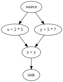
A computation graph for (2 x 5) + (5 x 7). Each node is an operation and each edge carries a value forward; backpropagation walks the same edges in reverse, multiplying local derivatives as it goes. Diagram by BrentPrinciple, CC BY-SA 4.0, via Wikimedia Commons.
Start with a computational graph. A graph is a directed acyclic graph whose nodes are operations and whose edges carry values. The forward pass computes each node’s output from its inputs, moving from the inputs to the loss. For a neural network with layers \(h^{(l)}\), the forward pass is just a sequence of functions: \(h^{(l)} = \sigma(W^{(l)} h^{(l-1)} + b^{(l)})\), where \(W^{(l)}\) is the weight matrix at layer \(l\), \(b^{(l)}\) is the bias, and \(\sigma\) is an activation function such as the logistic sigmoid or the rectified linear unit. The loss \(L\) is a scalar function of the final output. Training means finding weights that minimize \(L\).
The gradient \(\partial L / \partial W^{(l)}\) is what we need. The chain rule says that to compute it, we multiply together the derivatives along the path from \(L\) back to \(W^{(l)}\). For a deep network, there are many such paths, and the number of paths grows exponentially with depth if you think of them separately. Backprop avoids this blow-up by computing the derivatives once per node, in reverse order, and reusing them. Define the “error signal” at layer \(l\) as \(\delta^{(l)} = \partial L / \partial z^{(l)}\), where \(z^{(l)} = W^{(l)} h^{(l-1)} + b^{(l)}\) is the pre-activation. Then the error at the output is computed directly from the loss, and the error at each earlier layer is obtained from the error at the next layer by a single matrix multiplication with the transposed weights, multiplied elementwise by the derivative of the activation: \(\delta^{(l)} = \left( (W^{(l+1)})^\top \delta^{(l+1)} \right) \odot \sigma'(z^{(l)})\). The gradient with respect to the weights is then \(\partial L / \partial W^{(l)} = \delta^{(l)} (h^{(l-1)})^\top\).
That is the whole algorithm for a fully connected network. The forward pass stores the intermediate values, the backward pass consumes them, and each layer contributes one matrix multiplication to the backward sweep. The cost of the backward pass is comparable to the cost of the forward pass, which is the reason the reverse mode is so efficient. It is also why memory is often the binding constraint in practice: you have to store the activations from the forward pass to compute the backward pass, and for large models this dominates the memory budget.
It helps me to think about this in terms of Jacobians. Each node in the graph has a local Jacobian: the matrix of partial derivatives of its outputs with respect to its inputs. The chain rule says the total derivative of the loss with respect to any input is the product of the local Jacobians along the path. Reverse-mode differentiation multiplies these Jacobians from the loss backward, starting from a row vector (the gradient of the loss with respect to the output, which is a scalar), and therefore only ever performs matrix-vector products. Forward mode multiplies from the inputs forward, starting from a column vector, and computes the full Jacobian one column at a time. For a function with many inputs and one output, the reverse mode does one sweep. For a function with one input and many outputs, forward mode is better. Neural network training is almost always the first case, which is why reverse mode won.
The best short introduction to this that I know is Christopher Olah’s 201511ya essay, “Calculus on Computational Graphs: Backpropagation,” which works through the graph view with clear diagrams.16 I also recommend Michael Nielsen’s chapter on backpropagation from his online book on neural networks, which develops the same material in the index-heavy notation of the 1980s and is worth reading slowly.17 For a worked numerical example with real numbers, Matt 2015 step-by-step walkthrough is a good place to check your own calculations. And for an implementation that fits in a few hundred lines, Andrej Karpathy’s micrograd project shows that the whole machinery can be expressed as a scalar autodiff engine with a few dozen lines of core logic.
Here is the part I find most important, and the reason I think the textbook framing (“it’s just the chain rule”) is both true and misleading. Backprop is a particular order of computation. Once you see that, the other features follow. You can check gradients numerically by finite differences, which is slow and imprecise but independent of the algorithm, and this is how most of us debug a new layer. You can recompute activations rather than storing them, trading compute for memory, which is what gradient checkpointing does. You can define custom backward passes for operations whose derivatives are awkward to write out. And you can see why the algorithm breaks in certain situations: when the local Jacobians are very small or very large, the product over many layers vanishes or explodes, and that is the vanishing and exploding gradient problem in one sentence.
The phrase “leaky abstraction” comes from Karpathy’s widely read 2016 essay, “Yes you should understand backprop,” which argues that engineers who treat the framework as a black box will eventually be surprised by its failures.18 I think he is right, and I think the reason is precisely the order-of-computation point. If you know what is happening in the backward pass, you can reason about why a particular model is not training, why a particular loss function behaves badly, or why a particular normalization layer helps. If you do not, you are guessing. My own rule is that anyone who cannot write the backward pass of a two-layer network by hand should not be trusted to debug a deep one.
Why It Still Matters
It is fair to ask whether a 1970s numerical method and a 1980s training procedure still matter in an era of large transformers, mixture-of-experts layers, diffusion models, and reinforcement learning from human feedback. My answer is an emphatic yes, and the reason is that nearly every one of these systems is trained by some variant of gradient descent on a differentiable loss, with gradients computed by reverse-mode automatic differentiation. The architectures have changed enormously. The optimizer has changed in details (Adam and its descendants, learning-rate schedules, weight decay). The training algorithm is still backprop.
Schmidhuber claims that every mainstream deep learning framework implements Linnainmaa’s method, and I think that is essentially correct as a description of the computation, though it is a claim about implementation rather than about credit.19 PyTorch, JAX and TensorFlow all implement reverse-mode automatic differentiation over a computational graph, and the core idea is the one Linnainmaa wrote down. Whether they should be described as “Linnainmaa’s method” is partly a matter of taste, and I would not fight anyone who prefers to say “reverse-mode automatic differentiation” to avoid the priority question.
The other reason backprop still matters is that it defines the shape of the search. A model trained with backprop is one that can be improved by following gradients. That is both its power and its limitation. Gradients give you a local signal. They do not tell you about global structure unless the loss and the architecture encode it. They work best when the loss is differentiable, the data is abundant, and the model is large enough to have many paths by which the error can be reduced. When those conditions hold, backprop is hard to beat. When they fail, people reach for other tools, and that brings me to the part of the story that I find most intellectually open.
The Beyond-Backprop Literature
There is a substantial body of recent work that asks whether backpropagation is necessary, or at least whether it is the right algorithm for the job. I think this literature is worth taking seriously for three reasons. It is partly motivated by a legitimate question about biological plausibility. It is partly motivated by hardware constraints, since backprop requires storing activations and moving data in a way that is expensive on some chips. And it is partly motivated by the sheer intellectual pleasure of finding a different way to assign credit.
The biological plausibility question has a long history. The brain does not obviously implement backpropagation: neurons do not seem to transmit precise error signals backward along their axons, and the weight-transport problem, in which the backward pass needs the same weights as the forward pass, looks like a serious objection. A number of proposals try to address this. Predictive coding is one such framework, in which each layer predicts its inputs and learning is driven by local prediction errors, and there are arguments that predictive coding can approximate backprop under certain assumptions. A 2021 discussion on LessWrong and related work on unifying predictive coding with backprop made this connection explicit, and a 2019 review in Trends in Cognitive Sciences surveyed theories of error backpropagation in the brain.20 I have not opened the review in full for this essay, so I would not lean on its specific claims, but the overall direction is clear: the field is trying to find local learning rules that approximate the global gradient.
Hardware motivates a different set of proposals. Spiking neural networks, which communicate through discrete events in time, are attractive for energy efficiency, but they are awkward to train with standard gradient methods because the spike function is not differentiable. One response is to use surrogate gradients. Another is to compute exact gradients for event-based models, which is what a 2020 arXiv preprint titled “Event-Based Backpropagation can compute Exact Gradients for Spiking Neural Networks” (arXiv:200917ya.08378) claims to do.21 I think the exact-gradient approach is intellectually satisfying even if it is not yet the practical default, because it shows that the reverse computation can be extended to a domain that looked incompatible with it at first.
The meta-learning direction is more speculative. A 2020 preprint titled “Meta Learning Backpropagation And Improving It” (arXiv:201214ya.14905) explores whether the learning rule itself can be learned, so that the update computed from the forward activations is not fixed to backprop but is itself a parameterized function.22 I find this idea both exciting and slightly uncomfortable. It is exciting because it suggests that backprop might be one point in a larger space of learning rules, and that good rules could be discovered rather than designed. It is uncomfortable because the outer loop that learns the rule is itself trained with backprop, so the question of whether backprop is necessary becomes a question about what the outermost loop uses.
Then there are the more radical alternatives. The Forward-Forward algorithm, which Hinton proposed in 2022, replaces the backward pass with two forward passes, one on positive and one on negative data, and learns each layer locally with a goodness function.23 Direct feedback alignment, which replaces the transposed weights in the backward pass with fixed random matrices, shows that exact weight symmetry is not necessary for learning in some settings. A 2020 preprint on a photonic co-processor for direct feedback alignment (arXiv:201214ya.06373) is an example of how these ideas are being pushed toward specialized hardware.24 And a 2025 preprint titled “NoProp: Training Neural Networks without Full Back-propagation or Full Forward-propagation” (arXiv:2503.24322) proposes a method in which each layer is trained with a local denoising objective, with no global backward pass.25 I should note that the title of the NoProp preprint, as it appears on arXiv, is different from the version I saw in a discussion thread, which is a reminder to check primary sources.
I have to be careful about the most recent claims. I have seen references in recent community discussions to a line of work on pretraining transformers without backpropagation, and I have not been able to read the primary source for this essay, so I will not describe its results.26 I will say that the pattern is the same as before. Each new alternative is evaluated against backprop on some benchmark, and the verdict depends heavily on the benchmark, the scale, and the compute budget. So far, none of these alternatives has displaced backpropagation at the scale where most of the computation happens. Several have shown that the global backward pass is not strictly necessary for particular tasks, and that is interesting. But it is not the same as showing that a better algorithm exists for training the models we actually use.
My prediction, for what it is worth, is that backpropagation will remain the default for at least the next several years of large-scale training, and that the alternatives will matter most in three places: neuromorphic and analog hardware, where the cost of moving data for a global backward pass is prohibitive; biological modeling, where the question is what the brain does rather than what is most efficient; and settings where the loss is not easily differentiated end to end. In each of these, the alternatives are addressing a real constraint. In the standard data-center setting, backprop is already fast enough, and the main limitations are memory and communication, which people are working on with engineering rather than with new learning rules.
What I Think
Having gone through the history and the math, I want to state my view directly, because this is an essay and not a survey.
First, backpropagation is not really an invention of 198640ya, and the popular story that one group of researchers discovered it in that year is wrong. The reverse-mode computation is older than the neural network application by a decade or more, and the neural network application itself was developed in pieces by several people. The 198640ya paper deserves its reputation for making the idea legible and useful, not for originating it. I think a fair historian would give Linnainmaa, Werbos and the 198640ya authors substantial but different kinds of credit, and I would be cautious of anyone who tries to award the whole prize to one of them.
Second, the most useful way to understand backprop is as a particular order of computation over a differentiable graph, and not as a special rule for neural networks. This is why the “it’s just the chain rule” framing is both right and unhelpful. It is right that the mathematics is elementary. It is unhelpful because the elegance of the algorithm lies in the ordering, and the ordering is what determines memory use, numerical stability, and the kinds of failures you see in practice. Anyone who wants to train neural networks seriously should be able to write the backward pass by hand for a small model, and should be able to explain why the vanishing gradient problem is a consequence of multiplying many local Jacobians.
Third, the beyond-backprop literature is valuable, but it has not yet shown that backprop is the wrong algorithm for the systems we build. The biological plausibility arguments are important for neuroscience, and the hardware arguments are important for the next generation of chips. The meta-learning and local-learning proposals are intellectually interesting. But the empirical record so far is that backprop, combined with good architectures and enough data and compute, works better than its alternatives at the scale where most of the computation is done. I would be delighted to be proven wrong, and I think the people working on alternatives are doing the field a service by asking the question. But I would not bet against gradient descent on a differentiable loss for the foreseeable future.
Fourth, and most personally, I think the history of backpropagation is a good antidote to the view that progress in machine learning is driven by a few brilliant insights made by a few brilliant people. Backprop was a combination of a numerical method, a control-theory technique, a demonstration in a prestigious journal, a convolutional architecture, a set of hardware advances, and a lot of patient engineering that made deep networks trainable. Each of these pieces had its own history, and the algorithm we use today is the product of all of them. The priority fights are a reminder that credit is distributed and that the people who write the first clear statement of an idea do not always get the most recognition for it. That seems right to me, and it is a good reason to read the older literature.
Conclusion
Backpropagation is the algorithm that turned a set of mathematical observations into a practical method for learning from data. Its core is the chain rule, applied in a particular order that makes gradients cheap to compute. Its history runs from the calculus of the seventeenth century through the optimal control problems of the 1960s, the reverse-mode numerical work of Linnainmaa in 197056ya and 197650ya, the neural network application developed by Werbos in the 1970s and 1980s, the 198640ya demonstration by Rumelhart, Hinton and Williams, the convolutional architecture and real-world application of LeCun and coauthors in 198937ya, and the deep learning revival of the 2000s and 2010s. The priority disputes are real, but they are better understood as a story about how ideas become useful than as a contest with a single winner.
I still find the algorithm elegant, and I still think it is worth understanding deeply, even for people who will never implement it themselves. The alternatives are interesting, and some of them may matter a great deal in the coming years. But for now, when I call loss.backward(), I am invoking a computation that was first clearly written down by someone studying rounding error, and that became the engine of modern machine learning because a few later people realized what it could do. That is a strange and satisfying history, and I think it is worth knowing.
Further Reading
Gradient Descent Variants: the optimizers built on top of backpropagation
The Transformer Architecture: the architecture where most modern backpropagation actually runs
Convolutional Neural Networks: the weight-sharing idea that made backpropagation practical for images
Overfitting and Regularization: what happens when the learning goes too well
Mechanistic Interpretability: trying to read what backpropagation-trained networks actually learned
Calculus on Computational Graphs: Chris Olah’s visual explanation
Neural Networks and Deep Learning: Michael Nielsen’s chapter 2, a gentle derivation
Citation
Mert. 2026. “Backpropagation: The Chain Rule That Ate Machine Learning.” Journey of a Distracted Mind. journeyofadistractedmind.com/backpropagation
Rumelhart, David E., Geoffrey E. Hinton, and Ronald J. Williams. 198640ya. “Learning Representations by Back-Propagating Errors.” Nature 323: 533–536. doi:10.1038/323533a0