Gradient Descent and Its Variants

Mert

Gradient Descent and Its Variants

From vanilla SGD to Adam and beyond: the optimization algorithms that make neural network training possible, their motivations, failure modes, and why Adam won.

2026-04-06–2026-06-21 finished certainty: likely importance: 7

Gradient Descent and Its Variants

Gradient Descent and Its Variants

Here is something that still strikes me as slightly absurd. The entire edifice of modern deep learning, the thing that writes code and folds proteins and generates photorealistic video, rests on an algorithm a calculus student could derive: walk downhill. Compute a gradient, step in the opposite direction, repeat. That is the whole idea. Everything else is bookkeeping about how big the step should be and which direction “downhill” really means once you have a billion parameters and a loss surface no human will ever see.

I find that bookkeeping more interesting than it has any right to be. The history of optimization in deep learning is a chain of small, sharp fixes, each one patching a concrete failure of the method before it. Vanilla gradient descent is too slow, so we sample. Sampling oscillates, so we add momentum. Momentum uses one learning rate for everything, so we make it adaptive. Adaptive methods overfit the schedule, so we decouple the weight decay. None of these steps required a conceptual leap. Each one is the kind of thing that feels obvious in retrospect and took years to actually land.¹

This essay traces that chain from vanilla stochastic gradient descent through momentum, Nesterov acceleration, and the adaptive family that ends in Adam. I am not trying to catalog every optimizer ever published. I want to build intuition for why each variant exists, what it actually buys you, and when the choice matters at all. Because one of the running themes here, and one the practitioners who train these models for a living keep repeating, is that the optimizer often matters less than you would think.

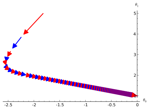
Gradient descent following the negative gradient downhill on a contour plot. Author: Eviatar Bach. License: CC0 (public domain), via Wikimedia Commons.

Vanilla Gradient Descent

The starting point is the most natural thing you could do. Given a loss function \(\mathcal{L}(\theta)\) and its gradient \(\nabla_\theta \mathcal{L}\), update the parameters in the direction that decreases the loss fastest:

\[\theta_{t+1} = \theta_t - \eta \nabla_\theta \mathcal{L}(\theta_t)\]

where \(\eta\) is the learning rate. This is batch gradient descent: compute the gradient over the entire dataset, take one step, repeat. For convex functions, this provably converges to the global minimum given a small enough learning rate. For the non-convex loss landscapes of neural networks, it converges to something, usually a local minimum or a saddle point.²

The problem with batch gradient descent is obvious the moment you try to use it. Computing the gradient over the entire dataset for each single step is grotesquely expensive. For ImageNet, that means feeding all 1.2 million images through the network just to nudge the weights once. You would run out of patience long before the model learned anything. So nobody does this. The first variant is not really a clever improvement, it is a concession to reality.

Stochastic Gradient Descent

Stochastic gradient descent, SGD, estimates the gradient from a small random mini-batch of size \(B\) instead of the full dataset:

\[\theta_{t+1} = \theta_t - \eta \frac{1}{B} \sum_{i \in \text{batch}} \nabla_\theta \mathcal{L}_i(\theta_t)\]

The mini-batch gradient is a noisy but unbiased estimator of the true gradient. On average it points the right way, but any individual estimate is wrong. And here is the part I find genuinely lovely: the noise is not a defect you tolerate, it is a feature you exploit. The randomness helps the optimizer escape shallow local minima and saddle points, and it acts as an implicit regularizer that improves how well the final model generalizes.³

This noise-as-feature idea shows up constantly once you start looking for it. One commenter on Hacker News, writing under the handle spi about training a base model on a single consumer GPU, put the batch-size tradeoff in plain terms: “In the very short term, smaller batch size is typically better just because you need a certain amount of gradient updates to move away from the original random, hence pretty terrible, weight distribution. Larger batch size gives a steadier, but slower, convergence, so it’s hard to say for sure what is better for a given compute budget.” That is the whole tension in one breath. More noise means more, scrappier updates that get you off the starting line fast. Less noise means smoother but slower progress.

Typical batch sizes run from 32 to a few thousand, though work on large-batch training shows you can push much higher if you scale the learning rate to match. SGD, plain and noisy, has trained most of the models that matter in the history of the field. But it has two weaknesses that the rest of this essay is really about. It oscillates badly in directions where the loss surface curves sharply, and it treats every parameter identically regardless of that parameter’s gradient history. The variants below each attack one of these.

Momentum

The oscillation problem is easiest to picture in a long, narrow valley, a loss surface shaped like a canyon. The gradient points mostly across the valley, down the steep walls, rather than along the floor toward the actual minimum. Plain SGD ricochets back and forth between the walls while making painfully slow progress down the length of the canyon. It is doing a lot of work to go almost nowhere.

Momentum fixes this by accumulating a velocity vector instead of stepping directly along the current gradient:

\[v_{t+1} = \mu v_t + \nabla_\theta \mathcal{L}(\theta_t)\] \[\theta_{t+1} = \theta_t - \eta v_{t+1}\]

where \(\mu \in [0, 1)\) is the momentum coefficient, almost always 0.9. The velocity is a running accumulation of past gradients. In the canyon, the cross-valley components alternate sign on each step and cancel out, while the along-valley components all point the same way and reinforce each other. The optimizer builds up speed in the consistent direction and damps the wasteful side-to-side motion.⁴

Momentum is so reliably helpful that when a practitioner says they trained a model with “SGD,” they almost always mean SGD with momentum 0.9 and some learning rate schedule, typically cosine annealing or step decay. Plain SGD with no momentum is mostly a teaching tool. The momentum version is the one that does the work.

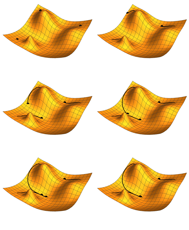
A loss surface visualized as a contour plot, with the optimizer’s path descending toward the minimum. Author: Jacopo Bertolotti. License: CC0 (public domain), via Wikimedia Commons.

Nesterov Accelerated Gradient

Nesterov momentum, often abbreviated NAG, is a small but genuinely clever modification. Standard momentum computes the gradient at your current position, then adds the accumulated velocity. Nesterov flips the order: first take the momentum step to a “lookahead” position, then compute the gradient there, and correct from that vantage point.

\[v_{t+1} = \mu v_t + \nabla_\theta \mathcal{L}(\theta_t - \eta \mu v_t)\] \[\theta_{t+1} = \theta_t - \eta v_{t+1}\]

The intuition I keep coming back to: standard momentum is throwing a ball and seeing where it lands. Nesterov is throwing the ball, peeking at where it is about to end up, and adjusting mid-flight. That foresight lets it slow down before overshooting rather than after, which gives better convergence on convex problems and a modest but real benefit in practice.⁵

For convex functions, Nesterov hits the optimal first-order convergence rate of \(O(1/t^2)\) against \(O(1/t)\) for plain gradient descent, a result from Nesterov1983. For non-convex neural network training the theoretical guarantee evaporates, and the practical gain is real but small. This is a recurring pattern in optimization: the clean theorems live in convex-land, and the messy empirical world keeps most of the benefit anyway, just with no proof attached.

The Adaptive Methods

Momentum solves oscillation, but every method so far still uses a single global learning rate for all parameters at once. That is a real limitation. Imagine a network processing language. The embedding for the word “the” gets a gradient on nearly every batch, while the embedding for some rare technical term gets updated only when that term happens to appear, maybe once in ten thousand steps. Forcing both to share a learning rate is clearly wrong. The frequent parameter wants small, careful steps; the rare one wants to move decisively on the few signals it gets.

AdaGrad

AdaGrad (Duchi et al 2011) was the first adaptive method to see wide use. It keeps a per-parameter running sum of squared gradients and uses it to scale each parameter’s learning rate individually:

\[G_{t+1} = G_t + g_t^2\] \[\theta_{t+1} = \theta_t - \frac{\eta}{\sqrt{G_{t+1}} + \epsilon} g_t\]

where \(g_t = \nabla_\theta \mathcal{L}(\theta_t)\) and \(\epsilon\) is a tiny constant to avoid dividing by zero. Parameters with a history of large gradients get their learning rate shrunk; parameters that rarely see a large gradient keep a big one. For the rare-word problem above, this is exactly right, and AdaGrad works beautifully on sparse problems.

But it has a fatal flaw for deep learning. \(G_t\) is a sum, and a sum of squares only ever grows. The effective learning rate marches monotonically toward zero and eventually becomes so small that learning stops, often long before the model has actually converged. For the dense, persistent gradients typical of neural networks, AdaGrad strangles itself. It is a cautionary tale about accumulators with no forgetting.

RMSProp

RMSProp (Hinton, 2012_14ya) fixes AdaGrad’s runaway accumulation with one small change: replace the sum with an exponential moving average.

\[G_{t+1} = \beta G_t + (1 - \beta) g_t^2\] \[\theta_{t+1} = \theta_t - \frac{\eta}{\sqrt{G_{t+1}} + \epsilon} g_t\]

with \(\beta\) usually 0.999. Now the running estimate has a finite memory. Old gradients decay away, so the effective learning rate can go down and back up, tracking the recent gradient statistics instead of the entire history. The strangling problem disappears.

There is a wonderful piece of academic-culture trivia buried here. RMSProp was never published in a paper. It appeared in the slides for Hinton’s Coursera course and spread purely by word of mouth and citation-to-the-slides. It went on to become one of the most-used optimizers in the field anyway. People on Hacker News still argue about what that says. In a thread on academic gatekeeping, one commenter noted that the Adam paper, RMSProp’s direct successor, “was published at ICLR, a top conference,” and another, Al-Khwarizmi, pushed back on the idea that peer review is essential by pointing exactly at cases like this: some of the most influential work, like the GPT-2 report, never went through a traditional venue at all. RMSProp is the cleaner example. A lecture slide became infrastructure.⁶

Adam

Adam (Kingma and Ba2015) is the one that won, and it won by combining momentum and RMSProp into a single update. It tracks exponential moving averages of both the first moment (the mean of the gradient, which is momentum) and the second moment (the uncentered variance, which is RMSProp):

\[m_{t+1} = \beta_1 m_t + (1 - \beta_1) g_t\] \[v_{t+1} = \beta_2 v_t + (1 - \beta_2) g_t^2\]

with a bias correction to undo the fact that both averages start at zero and are biased toward zero early in training:

\[\hat{m}_{t+1} = \frac{m_{t+1}}{1 - \beta_1^{t+1}}, \quad \hat{v}_{t+1} = \frac{v_{t+1}}{1 - \beta_2^{t+1}}\]

\[\theta_{t+1} = \theta_t - \frac{\eta}{\sqrt{\hat{v}_{t+1}} + \epsilon} \hat{m}_{t+1}\]

The default hyperparameters, \(\beta_1 = 0.9\), \(\beta_2 = 0.999\), \(\epsilon = 10^{-8}\), work across a startling range of problems with no tuning at all.⁷ There is a nice intuition for what Adam is doing that I picked up from a Hacker News comment by yobbo: “Adam functions as a low-pass filter (and/or compressor) on the gradient. It filters out noise, which is wild during start of training. This is basically what all optimizers achieve in various ways, including momentum.” That framing stuck with me. The second-moment term divides out the scale of each parameter’s gradient, so noisy, high-variance directions get damped and clean, consistent ones get through. Adam is a signal-conditioning device wearing an optimizer’s clothes.

The same commenter flagged the cost, which is worth keeping in mind: “Adam uses several times more memory, and is slower, than momentum or just SGD. That’s reason to not use if not needed.” Adam stores two extra values per parameter, the first and second moment. For a model with billions of parameters, that optimizer state can dwarf the model itself in memory, which is why so much of the engineering around training huge models is really about managing Adam’s footprint.

Adam’s Known Issues

Adam won, but it is not flawless, and the flaws matter once you move past toy problems.

The generalization gap. Wilson et al 2017 showed that SGD with momentum often generalizes better than Adam on vision tasks, even when Adam reaches a lower training loss. The adaptive scaling seems to steer toward solutions that fit the training set well but transfer slightly worse. This is a big part of why a lot of competitive computer vision work still trains with plain SGD.
Weight decay done wrong. The original Adam paper folded L2 regularization into the gradient, which sounds harmless but is not. Because Adam then scales that combined quantity by the adaptive denominator, the regularization strength ends up coupled to each parameter’s gradient history in a way nobody intended. Loshchilov and Hutter2019 diagnosed this and proposed AdamW, which decouples weight decay from the gradient update entirely. AdamW is now the standard for training Transformers and large language models. If you train an LLM today, you almost certainly use AdamW and may not even realize the “W” is fixing a years-old bug.
It can fail to converge. Reddi et al 2018 constructed simple convex problems where Adam provably diverges, because the exponential moving average can forget a large, informative gradient too quickly. They proposed AMSGrad as a patch. In practice AMSGrad rarely beats plain Adam on real problems, so it never caught on, which is its own small lesson about the gap between worst-case theory and average-case engineering.
Epsilon sensitivity. For models with very sparse or very large gradients, language models at scale being the obvious case, the default \(\epsilon = 10^{-8}\) can cause instability. Bumping it to \(10^{-6}\) or higher is a common, slightly embarrassing fix that works more often than it should.

The practical takeaway is boring and reliable: use AdamW for Transformers and language models, and reach for SGD with momentum on vision tasks or anywhere you can afford to tune the learning rate by hand and want the last point of generalization.

Does the Optimizer Even Matter?

Here is the uncomfortable thing I have come to believe after reading enough of these papers and enough practitioner war stories: for most people, on most problems, the choice of optimizer matters far less than the amount of attention the field pays to it. The learning rate matters enormously. The optimizer, once you have picked a reasonable one, mostly does not.

This is not just my read. The people training real models at scale say it constantly. In a thread about deep learning frameworks, a practitioner posting as m0zg laid it out flatly: “Most SOTA models in my field are trained with SGD+momentum, super primitive stuff.” In the same breath they noted that “current optimizer research seems to have stalled, so people focus on training with huge batches and stuff like that.” That is a striking admission from someone shipping state-of-the-art results. The fancy optimizer is not where the wins are. The wins are in data, scale, and the unglamorous engineering of getting gradients across a cluster.

There is a deeper version of this discomfort. We do not really have a theory telling us which optimizer to use; we have a decade of accumulated folklore. A commenter named janalsncm put it well in a discussion of new architectures: “it should count for something that we’ve spent the last 20 years ironing out standard hacks to get NNs working. Someday we will hopefully have some theoretical grounding for basic things like network shape and size, optimizer, learning rate schedule, etc. Until that time we will be stuck using empirical methods (read: trial and error).” That is exactly the state of the art. AdamW with cosine decay is not a derivation, it is a Schelling point, the configuration enough people found works well enough that everyone now starts there to avoid wasting compute rediscovering it.

I do not say this to be cynical. The folklore is good. It is the compressed result of millions of GPU-hours of collective trial and error, and it saves every newcomer from repeating that search. But it is worth being honest that when you type AdamW into your training script, you are not invoking a theorem. You are trusting a tradition. And the most useful skill, the one the practitioners keep pointing at, is not knowing the update rules cold. It is knowing how to sweep a learning rate.

Learning Rate Schedules

Which brings us to the hyperparameter that actually earns its reputation. The learning rate \(\eta\) is the single most important knob in neural network training, and no fixed value is right for the whole run. Early on you want large steps to cover ground fast. Later you want small steps to settle precisely into a minimum without bouncing back out. That tension is what learning rate schedules resolve.

The common shapes:

Step decay. Drop the learning rate by a fixed factor, often 10x, at preset epochs. Crude, effective, still widely used.
Cosine annealing. Glide the learning rate down a cosine curve from a peak to near zero. This is the default for most Transformer training.
Linear warmup then decay. Start tiny, ramp linearly up to the peak over a few thousand steps, then decay. Standard for large language models, and the warmup is not optional.⁸
Cyclical learning rates. Oscillate between bounds instead of monotonically decreasing. Periodically “shaking” the optimizer can knock it out of a mediocre minimum into a better one.

There is also active research into making the schedule disappear entirely. A recent Show HN post for a schedule-free Lion variant captured the frustration that motivates it. The author, quantosaurus, described struggling “to stabilize training by using countless learning-rate schedulers, gradient clippers and normalizers” until they built something that needed none of them. Whether schedule-free methods hold up broadly is still open, but the impulse is telling. The schedule is the part everyone hates tuning, so of course people keep trying to automate it away.

The 1cycle Policy and Super-Convergence

Smith and Topin2018 demonstrated something they called “super-convergence”: training to equivalent accuracy in dramatically fewer epochs by running a single cycle of the learning rate up to an aggressive peak and back down. The mechanism is that large learning rates act as a regularizer, the big noisy steps prevent the model from settling into sharp overfit minima, and one well-timed aggressive cycle squeezes the most out of that effect.

The 1cycle policy ramps the learning rate from peak/25 up to the peak over the first 30 percent of training, then cosine-anneals down to peak/10000 over the rest. On some problems it cuts training time by 5 to 10x. Fast.ai popularized it, and it shines especially for fine-tuning and transfer learning. It is one of those tricks that sounds too good to be true and turns out to be solidly empirically grounded, which is roughly the motto of this entire field.

Second-Order Methods and Beyond

Everything above is a first-order method: it uses only the gradient, the first derivative. In principle you can do far better with second-order information, the Hessian matrix of second derivatives, which describes the local curvature. Newton’s method is the textbook example:

\[\theta_{t+1} = \theta_t - H^{-1} \nabla_\theta \mathcal{L}\]

Curvature tells you not just which way is downhill but how the slope is changing, which in theory lets you take much smarter steps. The catch is brutal. The Hessian for a model with \(N\) parameters is an \(N \times N\) matrix. For a billion-parameter model that is \(10^{18}\) entries, which you can neither compute nor store nor invert. So pure second-order methods are a non-starter at scale, and the research is all about cheap approximations: L-BFGS, K-FAC, and Shampoo, which try to capture useful curvature information without the full matrix.⁹

A nice way to close the loop: Adam is already a crude, implicit second-order method. The second-moment estimate \(v_t\) is a diagonal approximation of the Hessian, one number of curvature per parameter instead of the full matrix. That is a big part of why the adaptive methods punch so far above their formal first-order weight. They are sneaking curvature in through the back door, cheaply enough to actually run.

Practical Summary

If you are starting a new project and want the short version, here is what a decade of folklore distills to:

Default. AdamW with linear warmup and cosine decay. \(\beta_1 = 0.9\), \(\beta_2 = 0.999\), weight decay around 0.01, peak learning rate somewhere from \(10^{-4}\) to \(3 \times 10^{-4}\). This will train almost anything tolerably.
Vision. SGD with momentum 0.9 plus step or cosine decay is competitive and often generalizes a hair better. Learning rate around 0.1 at batch size 256.
Fine-tuning. Lower the learning rate to the \(10^{-5}\) range, shorten the warmup, and consider the 1cycle policy.
When in doubt, sweep the learning rate on a log scale. This is the single highest-value thing you can do, and it matters more than which optimizer you picked.

The landscape keeps moving. Lion, Sophia, and other recent proposals show real gains in specific settings, and some of them may eventually become the new default. But the Adam family is still the bedrock, and understanding why it works, and why a noisy downhill walk plus a few decades of patching turned into the engine of modern AI, is most of what you need to understand how neural networks learn at all.