Convolutional Neural Networks
From Hubel and Wiesel’s cat experiments to ResNet-152: how the convolution operation, weight sharing, and hierarchical feature extraction gave machines the ability to see.
- Convolutional Neural Networks
- The Biological Inspiration
- The Convolution Operation
- Pooling and Downsampling
- LeNet: Where It All Started
- AlexNet: the Revolution
- VGGNet: Depth through Simplicity
- GoogLeNet and Inception: Going Wider
- ResNet: Breaking the Depth Barrier
- What the Network Actually Learns
- Then The Transformers Showed Up
- So Does the Convolution Still Matter?
- Sources and Further Reading
Convolutional Neural Networks
The idea that you could teach a computer to see by showing it millions of labeled images and letting gradient descent figure out the rest seemed absurd for most of the history of computer vision. For decades, the dominant approach was to handcraft features: SIFT, HOG, Gabor filters, edge detectors, all painstakingly designed by researchers who understood optics and geometry. The features were fed into classifiers like support vector machines or random forests. This pipeline worked, sort of. It was good enough to detect faces in point-and-shoot cameras and read zip codes off envelopes. But it had a hard ceiling, because the features were fixed. No matter how clever the classifier, it could only work with the representations a human had handed it.1
Convolutional neural networks broke through that ceiling by learning the features themselves. Instead of a human deciding that edges and corners and textures are the right primitives, the network discovers, through backpropagation and millions of training examples, that early layers should detect edges, middle layers should detect textures and parts, and deep layers should detect objects and scenes. This hierarchical feature learning is the central insight of the CNN, and it turned out to be one of the most important ideas in the history of machine learning.
I want to trace that idea from a pair of cats in a Baltimore lab to a network that beat humans at recognizing a thousand kinds of objects, and then ask the question that hangs over the whole field right now: now that Transformers can do vision too, does the convolution still matter? My honest answer is yes, but not for the reason most people give. The interesting part is why.
The Biological Inspiration
The story begins, as many good stories in neuroscience do, with cats. In 195967ya, David Hubel and Torsten Wiesel were recording from neurons in the primary visual cortex of anesthetized cats, trying to figure out what made these cells fire. The famous version of the story is that they got a response by accident: a glass slide they were sliding into a projector cast a faint moving edge across the screen, and a cell that had been silent suddenly started crackling. The cell did not care about dots of light. It cared about oriented edges moving through a small patch of the visual field.2
Out of years of this work came a picture of the visual system as a hierarchy. “Simple cells” respond to edges at a particular orientation in a specific location. “Complex cells” respond to the same oriented edge but tolerate some movement, so the edge can drift around within a region and the cell keeps firing. Local receptive fields, feature detection, a bit of tolerance for position. That is not a loose metaphor for a convolutional network. It is almost a blueprint.
The connection became architectural with Kunihiko Fukushima’s Neocognitron in 198046ya, which stacked alternating layers of “S-cells” (simple, feature-detecting) and “C-cells” (complex, position-tolerant). It could recognize handwritten characters with some translation invariance. What it lacked was a general way to learn its features. Some were hand-designed, and there was no clean credit-assignment algorithm to tune the whole stack from labeled examples. The Neocognitron was the skeleton. What it needed was backpropagation, and that would take another decade to arrive at the party.
There is a recurring HN argument that the field keeps rediscovering neuroscience after the fact. As one commenter put it, “Whenever AI makes a big advance the analog was already known by neuroscientists.”3 I am sympathetic to the eye-roll buried in that, but I think it gets the causality backwards for CNNs specifically. Hubel and Wiesel did not just happen to predict convolutions. Fukushima and later Yann LeCun read the neuroscience and deliberately built it in. The biology was an input, not a coincidence.
The Convolution Operation
A convolution is a mathematically tidy way to bake in two strong assumptions about images: locality and translation equivariance.4
Locality says a pixel’s meaning depends mostly on its neighbors, not on pixels clear across the image. A convolutional layer enforces this by restricting each neuron’s receptive field to a small spatial region, typically 3x3, 5x5, or 7x7 pixels. Compare that to a fully-connected layer, where every neuron touches every input. For a 224x224 color image, one fully-connected neuron would have 224 x 224 x 3 = 150,528 incoming weights. A 3x3 filter on the same input has 27. That gap is the whole game.
Translation equivariance says that if an object slides across the image, the network’s internal description of it should slide too. Convolutions get this through weight sharing: the same filter is dragged across every position. A cat-ear detector learned from the top-left corner automatically works in the bottom-right, because it is literally the same 27 numbers applied everywhere. Weight sharing is also why CNNs are not absurdly large. A single 3x3 filter on 3-channel input has 27 weights no matter how big the image gets.5
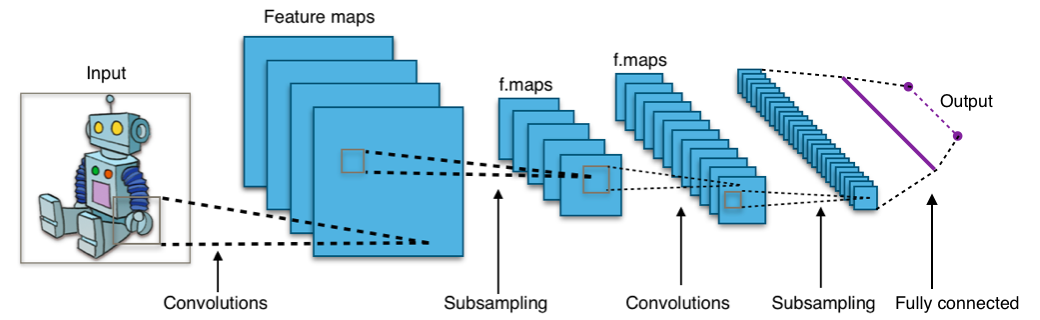
A typical convolutional neural network: alternating convolution and pooling stages reduce spatial size while growing feature depth, ending in fully-connected layers for classification. Image by Wikimedia user Aphex34, CC BY-SA 4.0.
A convolutional layer does not learn one filter, it learns many (commonly 64, 128, 256, or more), and each produces its own feature map, a 2D grid recording where that feature fired. So the output of a conv layer is a 3D tensor: height by width by number of filters. Stack these layers with nonlinear activations between them and you get a hierarchy of increasingly abstract features. The first layer’s filters end up looking like oriented edge detectors, which is exactly what Hubel and Wiesel found in V1, and nobody told the network to do that. It falls out of the data.
Pooling and Downsampling
Raw convolutions keep spatial resolution intact. But for classification you usually do not care where in the frame the cat is, only that a cat is present. That is the job of pooling. A pooling layer, classically max pooling over 2x2 regions with stride 2, halves each spatial dimension while keeping the strongest activation in each window. It buys a little translation invariance, since small shifts in the input leave the pooled output unchanged, and it cuts compute as the network deepens.6
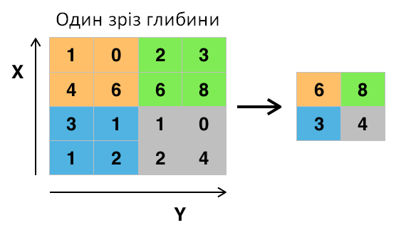
Max pooling with a 2x2 window and stride 2 keeps the largest value in each region, shrinking a 4x4 map to 2x2. Image by Wikimedia users Aphex34 and Olexa Riznyk, CC BY-SA 4.0.
Conv-then-pool, repeated, gives the classic CNN silhouette: spatial dimensions shrink while channel depth grows. An input of 224x224x3 might become 112x112x64 after the first block, then 56x56x128, then 28x28x256, and on down. The network trades spatial precision for semantic richness. By the deep layers, a single position in the feature map has a receptive field covering the whole image and stands for a high-level concept rather than a patch of texture.
Not everyone loves pooling, and the loudest skeptic is one of the people most responsible for deep learning existing at all. Geoffrey Hinton, in a Reddit AMA that gets quoted on HN to this day, said the quiet part out loud: “The pooling operation used in convolutional neural networks is a big mistake and the fact that it works so well is a disaster.”7 His complaint is that throwing away the precise location of a feature throws away the spatial relationships between features, which is how you end up with networks that will happily classify a face with the eyes and mouth scrambled. The field half-agreed with him in practice. Modern architectures quietly replaced max pooling with strided convolutions, which let the network learn its own downsampling instead of hardcoding “take the max.” Hinton’s deeper fix, capsule networks, never really caught on, but the critique stuck.
LeNet: Where It All Started
Yann LeCun and colleagues at AT&T Bell Labs built LeNet-5 in 199828ya, a 7-layer CNN for handwritten digit recognition that ran in production reading checks. It had every essential ingredient already: convolutional layers, pooling layers (they called it “subsampling”), and fully-connected layers at the end. It hit near-human accuracy on MNIST, which for 199828ya was genuinely impressive.8
And then nothing happened for fourteen years. This is the part of the story I find most instructive. LeNet was right. The architecture that would later conquer computer vision already existed, deployed, making money. But it worked on 32x32 grayscale digits, a long way from understanding a photograph of a dog on a beach. The hardware was not there, since practical GPU training was a decade away. The data was not there, since ImageNet would not exist until 200917ya. And the field’s attention was elsewhere, because support vector machines and kernel methods dominated the 2000s with cleaner theory and better small-data performance. CNNs went into a long winter. Having the right idea at the wrong time looks identical to having the wrong idea, right up until it doesn’t.
AlexNet: the Revolution
The winter ended abruptly in 201214ya. Alex Krizhevsky, Ilya Sutskever, and Geoffrey Hinton entered the ImageNet Large Scale Visual Recognition Challenge with AlexNet, a CNN that posted a top-5 error rate of 15.3% and beat the second-place entry’s 26.2% into the ground.9 The runner-up used handcrafted features. AlexNet learned its own. As one HN commenter summed it up years later, recalling the shock: “Relatively speaking they had about 40% fewer errors than anyone else. This is possibly the biggest result in computer vision the last five years.”10
Architecturally, AlexNet was LeNet scaled up and toughened for the real world: 8 layers (5 convolutional, 3 fully-connected), trained on 1.2 million ImageNet images across 1000 categories, on two NVIDIA GTX 580 GPUs with 3GB of memory each. The model was actually split across the two cards because it did not fit on one, which is why the original architecture diagram has that distinctive two-track shape. The key moves were practical rather than theoretical: ReLU activations for much faster training than sigmoid or tanh, dropout for regularization, aggressive data augmentation (random crops, horizontal flips, color jitter), and the willingness to throw GPUs at the problem. None of these were new on their own. The combination, at scale, was devastating.
There is a useful tension that AlexNet exposed and that has nagged at practitioners ever since. As one commenter described the rule of thumb for these networks: “95% of the computation time is spent in the conv layers, but 95% of the parameters are stored as the weights of the FC layers.”11 Convolutions are cheap in parameters but expensive in FLOPs, fully-connected layers are the reverse, and a lot of later architecture research is really about negotiating that split.
AlexNet did not just win a contest, it ended the argument about whether deep learning could do vision at all. Within a year the entire field had pivoted. Funding, talent, and conference papers all swung toward neural nets. I think it is the cleanest example we have of a single result resetting a research community’s priors overnight.
VGGNet: Depth through Simplicity
VGGNet (Simonyan and Zisserman, 201412ya) asked an almost stubbornly simple question: what if you just go deeper, with the most boring architecture imaginable? VGG used only 3x3 convolutions, the smallest filter that still captures left, right, up, down, and center, stacked 16 or 19 layers deep. The trick is that two stacked 3x3 layers see the same 5x5 region as a single 5x5 filter, but with fewer parameters and an extra nonlinearity in between.12
VGG-16 reached 7.3% top-5 error, a real jump over AlexNet. But its lasting contribution was legibility. The same 3x3 convolutions everywhere, double the filters after each pooling step, repeat. It was a template a grad student could hold in their head, modify, and build on, and its mid-network features became the default backbone for transfer learning in detection, segmentation, and style transfer for years. The cost was brutal: VGG-19 carried 144 million parameters and burned about 19.6 billion FLOPs per image. That was already scraping against what was practical, and it set up the tension the next architectures would attack.
GoogLeNet and Inception: Going Wider
Where VGG went deeper with uniform blocks, GoogLeNet (Szegedy et al., 201412ya) went wider. Its Inception module ran several filter sizes (1x1, 3x3, 5x5) plus pooling in parallel and concatenated the results, so the network could look at multiple spatial scales at once. Heavy use of 1x1 convolutions for dimensionality reduction kept the parameter count down to 6.8 million, roughly 20 times leaner than VGG, while still hitting 6.7% top-5 error with 22 layers.
The Inception line kept evolving into v2/v3 and v4, squeezing more out of ever more elaborate multi-branch designs. But the modules got harder to design and harder to reason about, and I think that complexity is exactly why the field’s attention soon swung to something you could explain in a sentence.
ResNet: Breaking the Depth Barrier
By 201511ya the field had hit a wall, and it was not the wall everyone expected. Stacking more layers onto a plain network made it worse, on both training and test data. This was not overfitting, which would show up as a train/test gap. It was an optimization failure. The loss landscape of a very deep plain network was simply too rugged for SGD to descend, and signals and gradients degraded as they passed through dozens of layers.
He et al. (201511ya) fixed it with residual connections. Instead of asking each block to learn a full mapping \(H(x)\), you ask it to learn a residual \(F(x) = H(x) - x\) and add the input back through a skip connection. If a layer has nothing useful to add, learning \(F(x) = 0\) leaves the input untouched, so depth can never actively hurt. The effect was startling: networks went to 50, 101, 152 layers, and each added layer reliably helped. ResNet-152 hit 3.57% top-5 error, past the human benchmark on that task.13 One HN commenter walking a newcomer through the lineage put it neatly: VGG showed depth was effective, “then you get ResNets with skip connections” and suddenly very deep was not just possible but easy.14
Skip connections turned out to be the most portable idea in modern deep learning. They are in the Transformer (see my notes on attention), in U-Nets for segmentation and inside most diffusion models, and in basically every deep architecture designed since. When an idea is simple enough to state in one breath and shows up everywhere afterward, that is usually the signature of something fundamental rather than a trick.
Post-ResNet: the Modern Landscape
After ResNet, CNN architecture research fanned out in a few directions, all chasing efficiency or expressiveness:
Efficient architectures. MobileNet (Howard et al., 2017) introduced depthwise separable convolutions, factoring a standard convolution into a spatial filter plus a 1x1 channel mixer and cutting compute 8 to 9 times with minimal accuracy loss. EfficientNet (Tan and Le, 2019) used neural architecture search to jointly scale depth, width, and resolution, reaching state-of-the-art accuracy with far fewer parameters.
Attention inside CNNs. Squeeze-and-Excitation Networks (Hu et al., 2018) added channel-wise attention, letting the network reweight which feature maps to trust. CBAM extended it to spatial attention.
Learned architectures. NASNet (Zoph et al., 2018) used reinforcement learning to discover convolutional cells. The found designs looked nothing like human-built ones and performed competitively, which is either humbling or thrilling depending on your mood.
ConvNeXt. Liu et al. (2022) took a plain ResNet and modernized it with tricks borrowed from Vision Transformers, including larger 7x7 kernels, fewer activations, and LayerNorm instead of BatchNorm. The result matched or beat the Swin Transformer on ImageNet. The convolution was not dead, it just needed a fresh coat of paint.
What the Network Actually Learns
One reason I trust CNNs more than most deep models is that you can look inside them and the insides make sense. Zeiler and Fergus (201313ya) built a deconvolutional technique to project activations back into pixel space, and what they found matched the theory almost too neatly. The first layer learns oriented edges and color blobs. The second learns corners, curves, and simple textures. By the middle layers you see honeycomb patterns, mesh, text. Near the top, whole object parts appear: dog faces, bird legs, wheels. The hierarchy that Hubel and Wiesel sketched in a cat’s visual cortex, and that Fukushima hand-built into the Neocognitron, falls out of backpropagation on its own when you give a CNN enough pictures.15
This interpretability is not just a nice-to-have. It is the thing that lets you debug a vision model. When a network confidently calls a husky a wolf, you can often trace it to a feature map that fired on snow in the background rather than the animal, a real failure mode documented in the LIME paper. Try getting that kind of legible diagnosis out of a fully-connected tangle.
The same property powers transfer learning, which is arguably the most economically important thing CNNs gave us. Because the early and middle features (edges, textures, parts) are generic across visual tasks, you can take a network trained on ImageNet, lop off the final classifier, and reuse the backbone for medical imaging, satellite photos, or defect detection on a factory line, with a few thousand labeled examples instead of a few million. Most applied computer vision for the past decade has been some flavor of “fine-tune a pretrained CNN.” It is not glamorous. It works absurdly well.
Then The Transformers Showed Up
For about eight years, “computer vision” and “convolutional neural network” were nearly synonymous. Then in 2020 a Google team published An Image Is Worth 16x16 Words and introduced the Vision Transformer, or ViT. The idea is almost insolently simple: chop an image into a grid of 16x16 patches, flatten each patch into a vector, treat the sequence of patches like words in a sentence, and feed it to a standard Transformer. No convolutions at all. At sufficient scale, it beat the best CNNs on ImageNet.16
I remember the reaction being a mix of awe and existential dread. The convolution, the one piece of hard-won architectural wisdom that everybody agreed was correct for images, turned out to be optional. You could throw it away and a generic sequence model would relearn whatever it needed from data. For a while it looked like the same story as natural language processing, where Transformers had already steamrolled the recurrent networks that came before.
But the ViT paper buried a crucial caveat that I think matters more than the headline. Vision Transformers only beat CNNs when trained on enormous datasets, like Google’s internal JFT-300M with 300 million images. On ImageNet alone (a mere 1.2 million images), plain ViTs lost to CNNs of comparable size. The reason is the concept that organizes this entire debate: inductive bias.
A CNN has locality and translation equivariance baked into its architecture. It does not need to learn that a cat in the corner is the same as a cat in the center, because weight sharing makes that true by construction. A Transformer assumes nothing. It has to learn that nearby patches are related, that translating an object should not change its identity, all of it, from data. When data is unlimited, that flexibility is an advantage, since the model can discover relationships a convolution would have forbidden. When data is scarce, the CNN’s built-in assumptions are a gift that saves it from relearning the obvious.
The Hacker News crowd, which contains a lot of people who actually train these things, zeroed in on exactly this. One commenter, chriskanan, put it cleanly: “Vision transformers have a more flexible hypothesis space, but they tend to have worse sample complexity than convolutional networks which have a strong architectural inductive bias.”17 Another, tourist_on_road, made the same point from the other side: “The fact there is no inductive bias inherent to transformers makes it difficult to train a decent model on small datasets from scratch.”18 And a third, algo_trader, summed up the tradeoff in a single line that I think is the whole essay in miniature: “you have to pay the price for losing the inductive bias of cnns.”19
So Does the Convolution Still Matter?
Here is where I land, after watching this argument run for a few years. The convolution matters, but we have learned to be precise about what it is good for, and that precision is the actual progress.
The field did not pick a winner. It blended. The Swin Transformer reintroduced locality and hierarchy into the Transformer by computing attention within local windows, which is a convolutional instinct wearing a Transformer costume. CvT and Compact Transformers literally bolt convolutions onto the front of a ViT to give it back some inductive bias and let it train on smaller datasets. And ConvNeXt ran the experiment in reverse, showing that if you modernize a pure CNN with the training recipe and a few design choices from Transformers, it keeps right up. When two approaches converge on each other’s tricks, the honest conclusion is that they were never really opponents. They are two points on a spectrum of how much structure you hardcode versus how much you let the model learn.
So the convolution still matters for the unglamorous, overwhelmingly common case: you do not have 300 million images. You have ten thousand chest X-rays, or a few thousand photos of manufacturing defects, or a modest video dataset. In that regime, the inductive bias of a CNN is not a limitation, it is the reason your model works at all. The pure-Transformer dream assumes a data budget that almost nobody outside a handful of large labs actually has.
The reason most people give for the convolution mattering is “it’s biologically inspired” or “it’s elegant.” I do not find those convincing on their own, because elegance does not pay rent and biology inspired plenty of dead ends too. The reason I find convincing is the sample-complexity argument. A convolution is a prior, a statement that says “I am willing to bet that images are local and translation-equivariant, and I will spend my limited data confirming the details rather than discovering the structure.” That bet has paid off so consistently, on so many real problems with realistic data budgets, that I would want a very good reason before giving it up. Most projects never get that reason, because most projects never get JFT-300M.
There is a deeper point hiding in all this about the bitter lesson, Rich Sutton’s argument that general methods leveraging computation eventually beat methods leveraging human knowledge. ViTs look like a clean win for the bitter lesson: less built-in structure, more compute and data, better results. But the qualifier “eventually” and the phrase “more data” are doing enormous work. For the slice of the world that has effectively infinite data and compute, the bitter lesson holds, and Transformers win. For everyone else, hand-designed inductive bias is still the most efficient way to turn a small dataset into a working model. The convolution is, among other things, a very good piece of compressed prior knowledge about what images are like. We figured out how to write that prior down in 198046ya, learned how to train it in 199828ya, learned it could win in 201214ya, and learned its exact limits in 2020. Knowing where a tool stops working is not a eulogy for it. It is what mastery looks like.
Sources and Further Reading
The foundational papers, in rough chronological order: Fukushima’s Neocognitron (198046ya), LeCun et al.’s LeNet (199828ya), Krizhevsky et al.’s AlexNet (201214ya), Simonyan and Zisserman’s VGG (201412ya), Szegedy et al.’s GoogLeNet (201412ya), He et al.’s ResNet (201511ya), and Dosovitskiy et al.’s Vision Transformer (2020). Related essays on this site: the Transformer architecture, attention mechanisms, backpropagation, the ResNet paper, and transfer learning.